A Hands-on Guide to Feature Engineering for Machine Learning

By Derrick Mwiti

A significant contributor to the success of applied machine learning is feature engineering. This article will take an immersive look at feature engineering and how it contributes to better machine learning models.

This article will cover the following topics:

what is feature engineering?
how to handle missing values
how to handle categorical features
normalizing of features
how to handle numerical/continuous features
how to create polynomial features
how you can work with date features
how to work with latitudes and longitudes

What is feature engineering?

The input to machine learning models usually consists of features and the target variable. The target is the item that the model is meant to predict, while features are the data points being used to make the predictions. Therefore, a feature is a numerical representation of data.

Viewing it from a Pandas data frame point of perspective, the features are the columns that one selects for their machine learning model. Rarely will you ever pass the raw features to the machine learning model. At the very least, the features have to be represented in a numerical form that the algorithms can accept. However, just converting the features into a numerical form doesn’t cut it. Enter feature engineering.

Feature engineering is the process of using domain knowledge to extract meaningful features from a dataset. The features result in machine learning models with higher accuracy. It is for this reason that machine learning engineers often consult domain experts.

For instance, when building a model to detect a particular disease, engineers will involve medical professionals in that field. This often results in better models because the engineer gains knowledge specific to the problem being solved. That said, how feature engineering is done will depend on the problem at hand.

For instance, image problems’ feature engineering will be different from the one done for natural language processing problems. Often the domain knowledge will be used to generate new features. For example, in the natural language process realm, a single statement is an observation, whereas the occurrence of a word could be a feature.

The problem that feature engineering solves

Before we get too far, it is important to note that feature engineering alone is not the holy grail. Other things work together to guarantee a well-performing model. Even with the best features, the choice of the algorithm will also determine how well the model performs.

It is also important to note that feature engineering isn’t one-size-fits-all, which means that you will have to engineer features depending on the problem at hand. That said, obtaining the optimal features will often lead to better performance even when using less complex models.

Feature engineering ensures that you get the best possible results from the data and algorithm. Therefore, feature engineering aims to enable you to get the most value from the data and algorithm being used.

Determining feature importance

It is vital to use the least and most important features when building models. Using the most optimal features will result in less complex models. Obtaining the most important features can be done by ranking the features. Certain algorithms will do the ranking out of the box. Some of these algorithms include:

You can disregard the other features and work with the most important features. You can also use features with high scores to create new features. Important features will often be highly correlated to the target, the item being predicted.

Process of feature engineering

Feature engineering can be thought of to happen in several steps. Let’s take an example of a model being built to predict the probability that a car insurance client will make a claim. Whether the person will make a claim is the item to be predicted. The predictor variables (or features could be):

the last time the person made a claim
their gender
their annual premium
their umbrella limit
their occupation
source of business
the person’s location
if the person has a health condition
whether the person has made a claim

Just to mention a few.

With that context, let’s look at how the feature engineering process would look like.

Feature creation

First, you will need to identify all the features that would be relevant in creating the model. This can be done through brainstorming and or consulting experts in the insurance field. As a result, you might identify important features that are not already included in the data. The absence of important features could also mean that you need to collect new data. Generally speaking, you cannot assume that the given data is sufficient to solve the problem in question.

Transformations

Data always needs to be transformed to a form acceptable by the machine learning algorithm being used. Here are a couple of items to consider:

some algorithms — for example, Sckit-learn algorithms– don’t accept data with missing values, whereas others like LightGBM can handle missing values by default. In neural networks, data with NANs will result in the loss being NAN as well. In such scenarios, you need to clean the data first.
some algorithms, such as Catboost, will handle categorical features by default while others will not.
distance-based algorithms such as neural networks will perform poorly when the data is not on the same scale. For such algorithms, the data first needs to be scaled before it is passed to the model.

Feature extraction

You can create new features by manipulating existing variables. This will result in variables that are more meaningful to the model. For instance, dates provided as a timestamp will not make sense to the algorithm. However, one can extract the following information that could make sense to the algorithm:

the hour of the day
the day of the week
the month
the day of the year

Just to mention a few.

Obviously, if the data is in text form; for instance, the day of the week, it will have to be represented in a numerical form.

Features can grow too quickly when certain methods such as feature combinations are applied. This phenomenon is known as feature explosion. You can avoid feature explosion through:

Sometimes you might be faced with data with too many features, often referred to as the curse of dimensionality. This requires the employment of dimensionality reduction techniques to reduce the number of features. A popular method for this is Principal component analysis (PCA).

Feature selection

The most naive thing to do is to use all the features from the dataset. There is nothing wrong with that if you just want to create a simple model and identify the most important features. However, this might not always be optimal, especially when working with a large dataset. Often, you will want to select the most optimal features because it will lead to fewer features and hence less computational resources needed.

In practice, you will employ the following information to come up with optimal features:

the literature on the domain of the problem.
testing the combination of various features.
using algorithms that automatically select the best features (more on this later)
good old common sense 😉

Feature engineering techniques

Let’s take a moment and look at how you can perform feature engineering in practice. Here are the techniques that will be covered:

imputing missing data
dealing with outliers
binning
log transformation
data scaling
one-hot encoding
handling categorical and numerical variables
creating polynomial features
dealing with geographical data
working with date data

In this example, obvious steps such as data loading are skipped. However, you can access the Google Colab notebook used here. The Kiva dataset is used for this exercise.

Let’s jump right in.

How to handle missing values

One of the main challenges of working with data is missing values. While some algorithms can handle missing values, others will throw errors.

Missing data imputation

The solution is to fill the missing values with statistical estimates. For example, the missing values can be filled with the:

mean
mode or
median

The first step is to compute the said statistical estimates. After that, you can use the `fillna` function to fill the missing values with the chosen estimates.

				
					mean_us = usa['loan_amount'].mean()
usa['loan_amount'] = usa['loan_amount'].fillna(median_us)

The same can be achieved using Scikit-learn. The `SimpleImputer` function can be used for this. The method requires:

the placeholder for the missing values, this could be `np.nan` or the string that was used to indicate missing values
the strategy that will be used to fill the values, for example, mean and mode

After instantiating the imputer, the next step is to fit and transform the column.

				
					
imp = SimpleImputer(missing_values=np.nan, strategy='mean')
usa['loan_amount'] = imp.fit_transform(usa[['loan_amount']])

You can also use the `IterativeImputer`. This function is still an experimental module in Scikit-learn. It estimates missing values by modeling each feature with the missing values as a function of other features in a round-robin fashion.

Here’s a quick example of how to implement it.

				
					
from sklearn.experimental import enable_iterative_imputer
from sklearn.impute import IterativeImputer
imp = IterativeImputer(max_iter=10, random_state=0)
imp.fit(usa[['loan_amount']])
usa['loan_amount'] = imp.transform(usa[['loan_amount']])

You can also impute categorical variables. For example, you can use the simple imputer to fill missing categories with the most frequent category.

The first step is to identify the most frequent category.

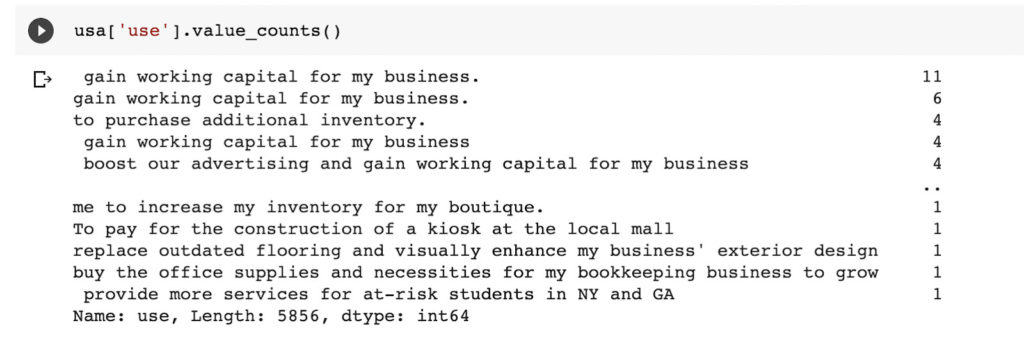
The next step is to fill the missing values with the most frequent category.

				
					
imp = SimpleImputer(strategy="most_frequent")
usa['use'] = imp.fit_transform(usa[['use']])

How to handle categorical features

Even after filling missing categories, you will need to convert them into a form that machine learning models can accept. This means that you have to choose a strategy that will be used to encode the category into a numerical representation. As you do so, you have to ensure that meaningful information is captured. Categorical features can be of two main types:

ordinal: these categories are ordered. For instance, high is bigger than medium and low when considering salary ranges, i.e., high > medium > low. The inverse is also true
non-ordinal: these categories have no order. For example, in the case of sectors, agriculture is not higher than housing.

You can choose to encode features manually. However, since there are open source tools for this, it is not necessary.

Label encoding

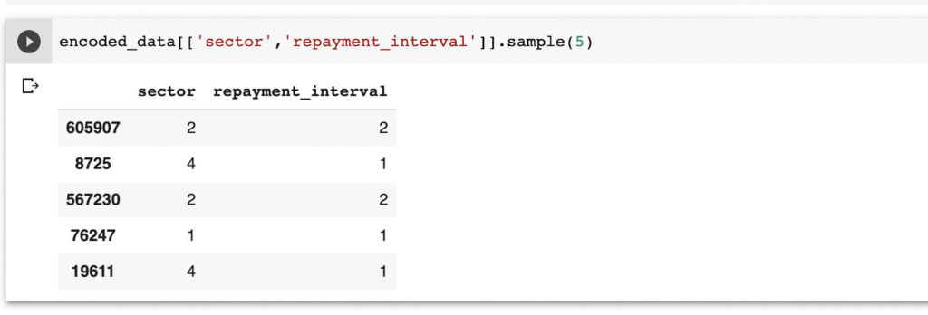
Label encoding is a category encoding strategy that maps each category to an integer. One popular tool for doing this is `category_encoders`. You’ll need to install it via `pip` or `conda`. Let’s look at how you can convert the repayment interval and sector categories from the Kaggle dataset.

The first step is to create a list of columns that you would like to convert.

				
					
cat_feats = ['sector','repayment_interval']

Next, create an instance of `OrdinalEncoder` with these features. The next step is to fit and transform the features.

				
					
import category_encoders as ce
encoder = ce.OrdinalEncoder(cols=cat_feats)
encoded_data = encoder.fit_transform(usa)

Here is a snapshot of the final result.

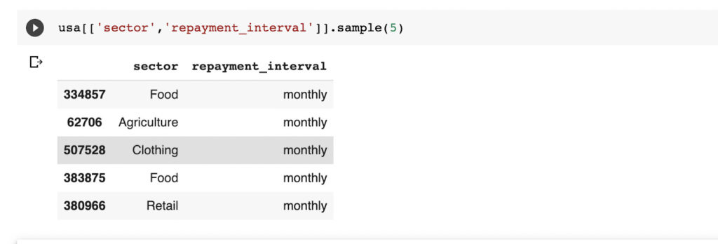
The screenshot below shows the columns before they were transformed.

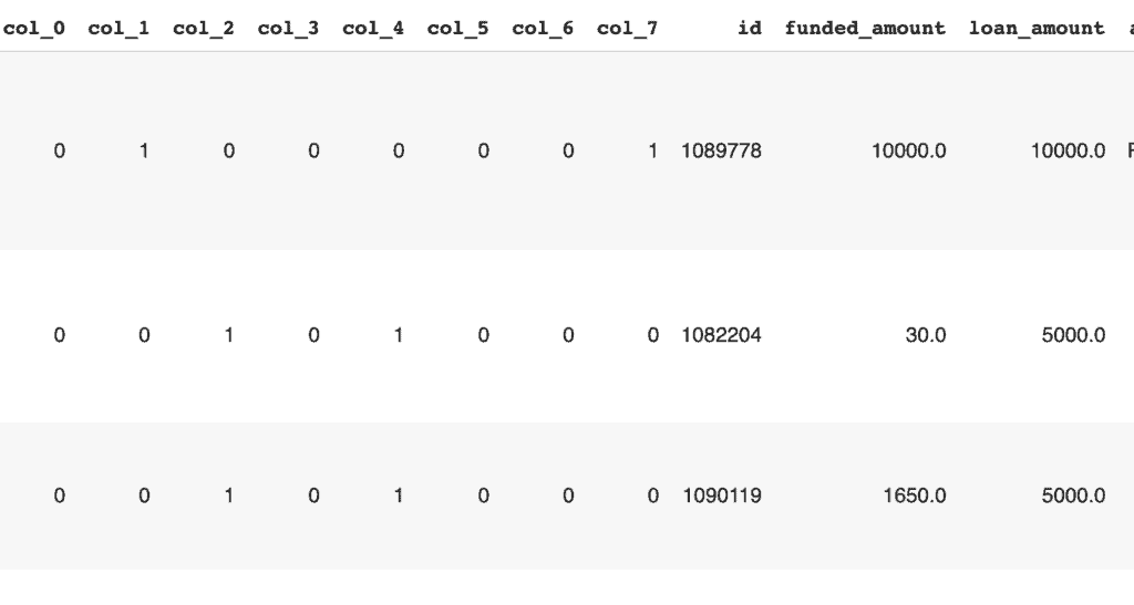
One-hot encoding

The next alternative is to use binaries to represent the categories. This results in the creation of a column for each category. When there are many categories, it leads to many new features. This can quickly result in the curse of dimensionality.

Category encoders can still be used for this kind of transformation.

				
					
one_hot = ce.OneHotEncoder(cols=cat_feats)
oe_data = one_hot.fit_transform(usa)

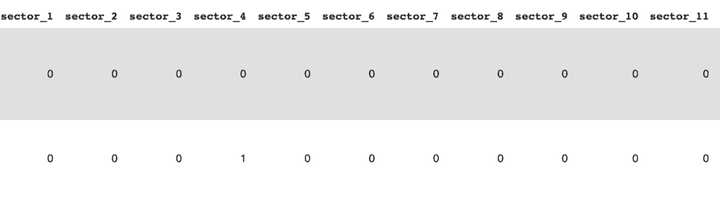
When performing one-hot encoding, it is usually a good idea to drop the first column to prevent multicollinearity. This can be illustrated using Pandas `get_dummies` function. Dropping the first level is specified by passing `drop_first=True`. This results in N-1 number of features.

				
					
data = pd.get_dummies(usa, drop_first=True,columns=cat_feats )

Hash encoding

Hash encoding can also be done using category encoders. It is a multivariate hashing implementation with configurable dimensionality. It doesn’t maintain a dictionary representation of the categories. It, therefore, doesn’t grow in size.

The hashing encoder requires:

the categorical columns to be encoded
the number of bits that will be used to represent the features

				
					
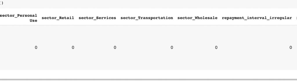
hash_enc = ce.HashingEncoder(cols=cat_feats, n_components=8)
hash_enc_data = hash_enc.fit_transform(usa)

How to handle numerical/continuous features

Numerical features also need to be processed to a form that guarantees optimal results when passed to an algorithm. Let’s take a look at some strategies that you can use to handle numerical data.

Feature scaling

Certain algorithms and neural networks require that the data is transformed into small numbers within a specific range. This is because the weights of neural nets, for example, are initially to very small numbers. The process of scaling the features is often also referred to as feature normalization.

Some common strategies for normalizing data are using the:

standard scaler: standardizes features by removing the mean and scaling to unit-variance
min max scaler: transforms the numerical values by scaling each feature to a given range; for example forcing all values to be between zero and one
robust scaler: scales the numerical values using statistics that are robust to outliers. It gets rid of the median and scales the data according to the quantile range

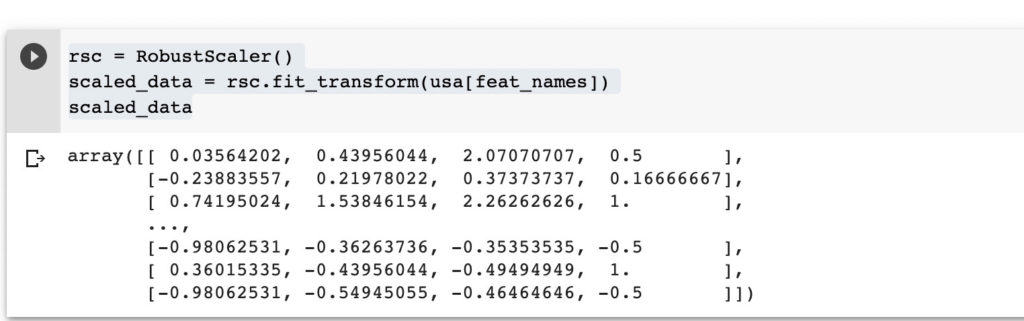
Here is an example of how you can transform data using the robust scaler. The other scalers can also be applied similarly.

The process of applying the scalers involves:

creating an instance of the scaler
fitting it to the data
transforming the data

				
					
rsc = RobustScaler()
scaled_data = rsc.fit_transform(usa[feat_names])
scaled_data

The scaler should never be fitted to the testing set because it will lead to data leakage. You should fit the scaler to the training set and then use the learned parameters to transform the testing set.

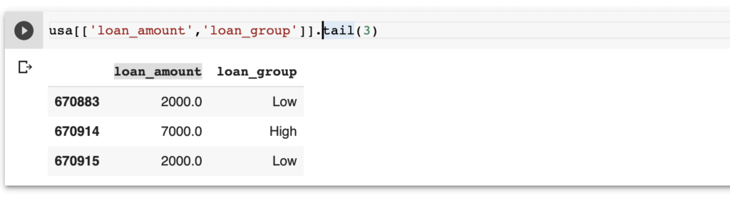
Converting numerical variables into discrete

You can also create numerical variables into discrete data. This can be done by creating bins from the numerical data. For example, given the loan amount in this data, you can create a new column indicating whether the loan was low, medium, or higher.

Bins can be created using the `cut` method from Pandas. It requires:

the data to be binned
the number of bins
the new labels

				
					
usa['loan_group'] = pd.cut(usa['loan_amount'], bins=3, labels=["Low", "Mid", "High"])

Here is the final result of the above transformation.

Log transformation

You can use log transformation to center data if it is skewed. When interpreting the results, you have to remember to take the exponent.

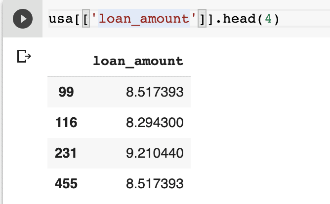
You can transform the data using NumPy’s `log1p` method. This implementation adds one to each number before taking the logarithm and prevents taking the log of zero. Taking the log of zero results in error.

				
					
usa['loan_amount'] =  np.log1p(usa['loan_amount'])

Creating polynomial features

Polynomial features are created by crossing two or more features. This creates a relationship between the independent variables. The relations could result in a model with less bias.

You can create these features using Scikit-learn’s `PolynomialFeatures`.

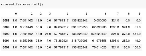
Let’s look at how you can create new features from the `loan_amount`, `term_in_months`, and `lender_count`. This is done by creating an instance of the `PolynomialFeatures` and then fitting it to the selected columns.

				
					
from sklearn.preprocessing import PolynomialFeatures

poly_feats = PolynomialFeatures()
columns_to_cross = ['loan_amount', 'term_in_months', 'lender_count']
crossed_features = poly_feats.fit_transform(usa[columns_to_cross].values)

crossed_features = pd.DataFrame(crossed_features)

Handling outliers

The easiest way to identify the presence of outliers is through visualization. Values falling outside the whiskers in a box plot are usually outliers.

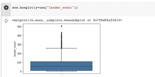
There are two common ways of dealing with outliers:

dropping all outlier values
capping the values to a certain maximum

You can experiment with the two and identify the one that results in a better model. A more reliable approach is to work with a domain expert to determine the best approach.

Grouping operations

You can also generate a new dataset through grouping operations. For instance, you can create a pivot table by aggregating the data based on the sum of the `loan amount` and selecting the `sectors` column. You can also select more than one column.

				
					
usa.pivot_table(index='day', columns=['sector'], values='funded_amount', aggfunc=np.sum, fill_value = 0)

Feature splitting

Sometimes you may be presented with data that would make more sense to a model if it was split. For example, you might have a movie’s name column that represents data in this form.

movie (2004)

In this case, you can split this single column into two columns; a movie name column and a year of release column. You should be able to do this with simple Python functions.

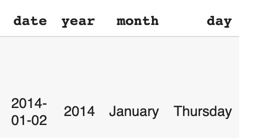
How to handle date features

When provided with date data, you can use it to generate more features such as the year, month, and day. This is something that you can easily do using Pandas. For example, here is how you would extract the year from the date.

				
					
def create_year(x):
    year = pd.DatetimeIndex(x).year 
    return year

usa['year'] = create_year(usa['date'])

Working with latitudes and longitudes

You can also generate new features when longitude and latitude data is provided. Libraries such as GeoJson and Geoopy can help with that. They can convert the geodata to physical addresses on a map.

In this article, let’s use Rising’s implementation to illustrate how you can use the longitude and latitude to compute the Manhattan distance, Haversine distance, and the bearing.

Given the latitude and longitude, you can compute the distance between two places.

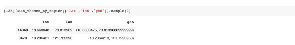
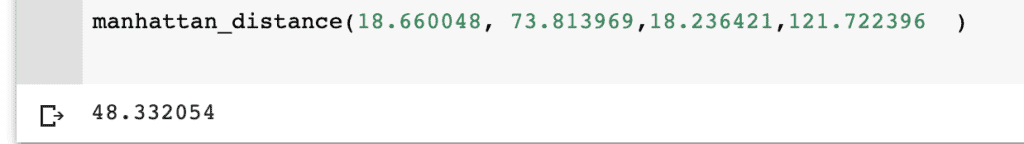
The distance can be computed using this function.

				
					
def manhattan_distance(lat1, lng1, lat2, lng2):
    a = np.abs(lat2 -lat1)
    b = np.abs(lng1 - lng2)
    return a + b
manhattan_distance(18.660048, 73.813969,18.236421,121.722396	)

The Haversine distance and the bearing are computed similarly. You can find the complete examples here.

Using domain knowledge

You can also use domain knowledge to generate new features. If you are not a domain expert in the problem you are trying to solve, consulting an expert will come in handy. For example, for the Kaggle data, you can create a new feature from the ratio of the lender count and the term in months.

Feature engineering automation

You can also use various tools to create new features automatically. One such tool is feature tools. It is an open-source library that generates new features from tables of related data. Since creating features manually can be cumbersome, employing automation tools can help hasten the process.

Here are a couple of concepts to note as far as using `featuretools` is concerned:

an `entity` refers to a single table or Pandas data frame. Each entity should have an index that is unique (without any duplicates)
An `EntitySet` defines a group of entities and the relationship between them

After installing `featuretools`, the next step is to import it and create an entity. `featuretools` can infer data types when creating an entity from a data frame. However, if you have categorical columns that are represented by integers, you need to inform feature tools to treat them as categories. That means you will have used the techniques for handling categorical data mentioned above before passing the data to feature tools

				
					
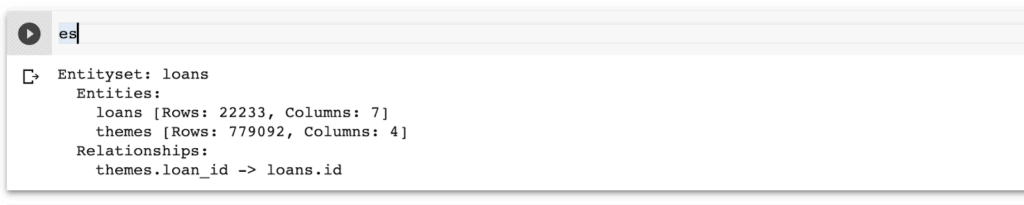
import featuretools as ft

es = ft.EntitySet(id="loans")
es = es.entity_from_dataframe(entity_id="loans", dataframe=encoded_data_loan_data, index="id",
           variable_types = { "sector": ft.variable_types.Categorical, 
                             "partner_id": ft.variable_types.Categorical,
                             "funded_amount": ft.variable_types.Numeric,
                             "loan_amount": ft.variable_types.Numeric,
                             "repayment_interval": ft.variable_types.Categorical })

The above code created an entity for the loan data frame. Let’s now do the same for the loan theme types.

				
					
es = es.entity_from_dataframe(entity_id = 'themes',
                              variable_types = {
                             "Loan Theme Type": ft.variable_types.Categorical,
                             "Partner ID": ft.variable_types.Categorical,
                              },
                              dataframe = encoded_data_themes, index = "index")

The loan id defines the relationship between the two tables. Each of the two has an id column. Let’s now use that to define the relationship in `featuretools`.

				
					
# Relationship between loans and themes
r_loan_themes = ft.Relationship(es['loans']['id'], es['themes']['loan_id'])
es = es.add_relationships([r_loan_themes])

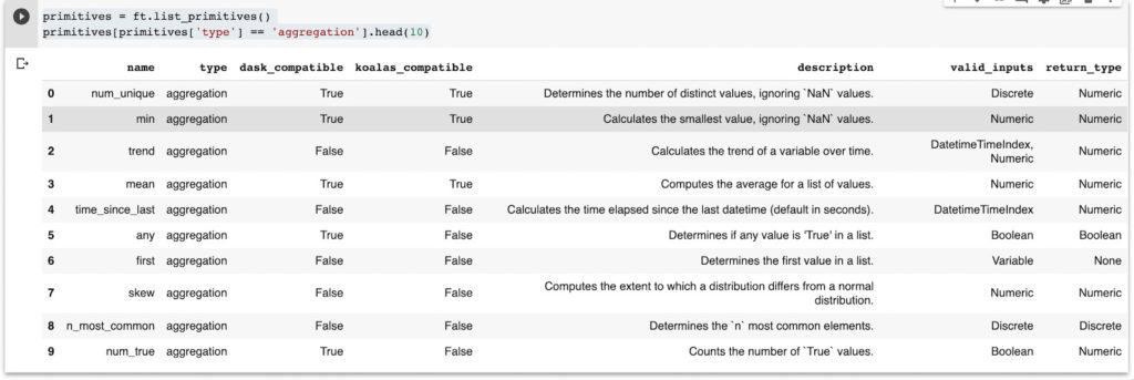
In `featuretools`, features are created using feature primitives. Feature primitives are computations that are applied to datasets to generate new features. Feature primitives are divided into two categories:

aggregation: these primitives take related input instances and return a single output, for example, the mean, count, etc. They are applied across a parent-child relationship in an entity set
transformation: these take one or more variables from an entity as input and output a new variable for that entity. They are usually applied to a single entity.

You can check the default aggregation primitives from feature tools as shown below:

				
					
primitives = ft.list_primitives()
primitives[primitives['type'] == 'aggregation'].head(10)

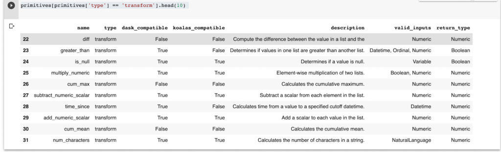
You can check transformation primitives similarly.

				
					
primitives[primitives['type'] == 'transform'].head(10)

`featuretools` generates new features through a process known as Deep Feature Synthesis (DFS). The `dfs` function from `featuretools` accepts the relationship between entities and the target entity, then generates new features. In this case, let’s create new features for the loan data frame. You can pass the primitives you would like to use or let `featuretools` use default ones.

				
					feature_matrix_loan, feature_names_loan = ft.dfs(
entityset = es, 
                                                target_entity = 'loans', 
 verbose = True,

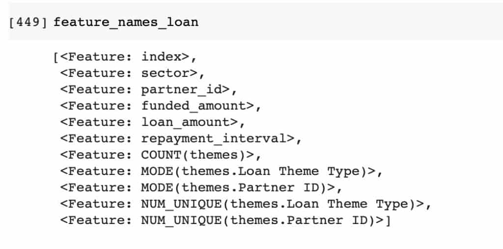
When the process is complete, you can check out the new data frame. If necessary, you can also export it to a file.

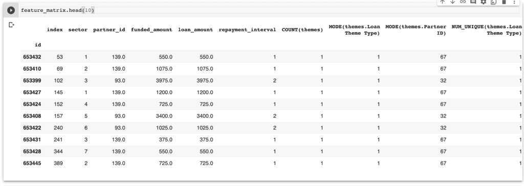
You can plot the new features to understand them. Here’s a snapshot of the generated features.

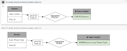
For instance, let’s visualize the features at indexes 6 and 7.

				
					
ft.graph_feature(feature_names_loan[6])
ft.graph_feature(feature_names_loan[7])

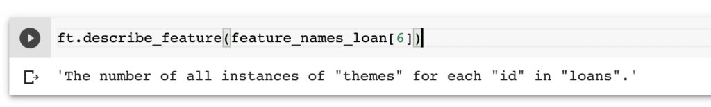
You can also generate an English explanation of a certain feature. For example, let’s take a look at the description of the feature at index 6.

				
					
ft.describe_feature(feature_names_loan[6])

Other feature engineering tools that you can look at include:

Best practices for feature engineering

You have covered so much ground so far. Let’s now take a step back and look at some best practices to have in mind when engineering features.

Indicator variables

Use indicator variables to incorporate vital information in the model. Here is how you would go about this:

creating indicator variables from thresholds. Let’s go back to that car insurance example again. For instance, let’s say that most accidents happen on the 20th day of the month. You can, for example, create a variable that indicates if the day of the month is greater than or equal to 20.
indicator variables for special events. In the case of car accidents, you can create flags to inform the algorithm if there are significant beer sale events at specific points of the year. It could be that there are more accidents and hence more insurance claims during these periods.
create indicator variables from multiple features. For example, if people who are alcoholics and are from a particular location make more claims, you can create an indicator variable for that.
indicator variable for group classes. In the data, you might have a field indicating how the client became a client of the insurance company. Some of these sources could be radio advertising, tv advertising, walk-in, website, etc. You may want to create a new flag that indicates if the client joined from a paid or a free source.

Interaction features

Other times you can create features from the interaction of two or more features. Here are some ways this can be applied:

the quotient of two features
the difference of two features
product of two features
the sum of two features

Feature representation

Feature representation simply means representing the same features differently. For instance:

extracting months, days, and hours from a timestamp
create categorical features from numerical data. For example, given the salary, you can create a new category with information such as low, medium, and high salary.
group classes that have very many categories but with a low count per class

External data

Bringing in external can lead to significant improvement in the performance of a model. For instance, when dealing with plant disease data, adding external data about weather patterns can improve model performance.

Error analysis

After training a model, you can check for errors such as misclassification and decide how to handle them. The goal is to understand why the model performed dismally. You can solve this problem by collecting more data and or creating new features. This would also be an excellent time to consult the domain experts again.

Final thoughts on feature engineering

Feature engineering can seem quite overwhelming in the beginning. However, it is a necessary step if you want to reap the benefits of a well-performing model. In this article, you have learned what feature engineering is and how you can apply it. Specifically, you have covered: