In this article, you are going to learn how to perform sentiment analysis, using different Machine Learning, NLP, and Deep Learning techniques in detail all using Python programming language.
At the end of the article, you will:
- Know what Sentiment Analysis is, its importance, and what it’s used for
- Different Natural Language Processing tools and tricks to preprocess and clean the textual data, so that it is ready to be fed to the model.
- Understanding the basics of the Naive Bayes algorithm and use it to classify the sentiment of a given input sentence using
- Using spaCy for sentiment analysis
- Custom NLP sentiment analyzer using Deep Learning with PyTorch
- Next steps with sentiment analysis
Introduction to Sentiment Analysis
Sentiment Analysis, also known as opinion mining is a special Natural Language Processing application that helps us identify whether the given data contains positive, negative, or neutral sentiment. This can be undertaken via machine learning or lexicon-based approaches. Sentiment Analysis helps to improve the customer experience, reduce employee turnover, build better products, and more. Almost every big and growing business is using Sentiment Analysis to automate it’s tasks and to maximize its profit.
The applications of sentiment analysis ranges from emotion recognition to text classification. The most common use case of sentiment analysis is on textual data where we use it to help a business monitor the sentiment of product reviews or customer feedback. Different social media platforms also use it to check the sentiment of the posts and if the sentiment of a post is very strong or violent, or below their threshold, they either delete it or hide it.
Since the rise of ecommerce and social media, applications that help business leaders automate the feedback process have been becoming particularly helpful. Sentiment Analysis is particularly seen often in retail. One of the main reasons that sentiment analysis is becoming popular for retail and technology businesses is because customers increasingly express their desires, thoughts, preferences and frustrations online. With sentiment analysis business owners can find out what their customers are saying and how they feel about the products they’re offering. Using social media, it’s now possible for retailers and tech companies to understand the sentiment of their customers in real time, finding out how they feel about the products on store shelves, store layouts and commercials. A sentiment analysis application could help quickly analyze the overall feedback of the product and determine whether customers were happy with it or not. Sentiment Analysis is also making its way into the Insurance industry which helps companies develop a pattern in insurance claims, settlement notes, etc. This helps prevent fraud and increases profits.
Despite diverse classification methods, sentiment analysis is not always accurate, as the language can be interpreted differently by computers and humans. Many jokes, sarcasm, irony, slang, or negations are typically understood correctly by humans, but can cause errors in computational analysis. Moreover, if the context of the speech is missing, the sentiment computed by the computer can be the opposite to the meaning
Some of the common examples of Sentiment Analysis are
- Customer Feedback
- Product Analysis
- Social Media Monitoring
- Brand Perception
- Emotion Recognition
- Chatbot reactions
- Voice of Employee
- Threat Detection etc.
Compared to 10 years ago, the ability to analyze sentiment has improved dramatically with the development in deep learning algorithms, availability of data, and high computational power via GPUs.
Sentiment analysis has been proven to save a lot of time and money for enterprises. It offers a way to quickly and automatically analyze large amounts of qualitative data and extract insights or results from it.
Different Types of Sentiment Analysis
There are different kinds of sentiment analysis and applications. This article will discuss 4 important types and popular use cases of Sentiment Analysis.
1. Fine-Grained Sentiment:
This type of analysis gives you an understanding of customer feedback. You can get precise results in terms of the polarity of the input. For example, you can label the reviews as
- Positive
- Very Positive
- Negative
- Very Negative
- Neutral
And you are able to interpret ratings, such as 5 stars = Very positive and so on.

Source: Pixabay
2. Intent Analysis
This is a special type of analysis that goes deeper than basic sentiment analysis, and can determine whether the data is a complaint, suggestion, query. You are also able to capture the overall intention behind the specific data.
There are many examples of intent analysis. For example, if you run an active social media page for your company and someone tags your page your intent analysis algorithm will quickly classify whether it is a question, suggestion, or someone just joking around. This can help improve social engagement and customer experience. Another example where intent analysis can be used is in determining SPAM. Many email services use this to automatically detect SPAM and send it into your SPAM folder. This drastically improves customer experience, and saves time.
3. Aspect Based
As this type of sentiment analysis allows you to analyze a specific aspect of the data. For example, let’s say you have launched a new perfume, and you want to analyze the user’s feedback to check which aspect of your product they liked the most. You can then find out whether they liked the packaging, or scent, or the price, etc.
4. Emotion Detection
This is one of the most commonly used sentiment analysis where we detect the emotion behind a sentence. We aim to detect whether the given sentence is happy, sad, frustrated, angry.
This can be helpful to give an overall review of the data/feedback whether the general emotion of the audience is happy, or sad based on your product.
Using Machine Learning and Deep Learning for Sentiment Analysis
In the below section, we are going to discuss how we can make our Sentiment Analysis application using Machine Learning algorithms, NLP tools, and Deep Learning. But before we jump into building the machine learning model, we need to learn how we are going to clean our textual data.
As you know the machine learning models do not accept textual data in raw format, you have to feed in numbers. To begin, you’ll need to learn how to clean your data and make it ready for our model. This involves a few different techniques and some tricks, which are going to be discussed in detail in the coming section.
Cleaning the textual data for Sentiment Analysis
The dataset we are going to use for sentiment analysis is the famous movie review dataset from Kaggle, on which we have to classify the sentiment of the Movie. This is an example of Fine Grained Sentiment Analysis, where we have to classify fine-grained labels for the movie reviews. The 5 given labels are
- negative
- somewhat negative
- neutral
- somewhat positive
- positive
You can download this dataset from here. You’ll simply have to log in and accept the competition to download the dataset.
But first, you should download the necessary libraries. You can download it via the following commands.
pip install contractions
pip install nltk
pip install autocorrect
Let’s import important libraries now.
#imports
import string # from some string manipulation tasks
import nltk # natural language toolkit
import re # regex
from string import punctuation # solving punctuation problems
from nltk.corpus import stopwords # stop words in sentences
from nltk.stem import WordNetLemmatizer # For stemming the sentence
from nltk.stem import SnowballStemmer # For stemming the sentence
from contractions import contractions_dict # to solve contractions
from autocorrect import Speller #correcting the spellings
So the basic steps involved in cleaning the data are
- Tokenization
- Converting the text from upper case to lower case
- Correcting the spelling mistakes
- Punctuation removal
- Number removal
- Stop words removal
- Normalization via lemmatization or stemming
Now let’s discuss all of these in detail. There are no standard sequences or standard steps that are involved. They vary from example to example. Let us now import the dataset, and analyze it to get a basic understanding of it.
import numpy as np
import pandas as pd
train_data = pd.read_csv('train.tsv', delimiter='\t', index_col = 'PhraseId')
Let’s see the head of the dataset to check it.
train_data.head() 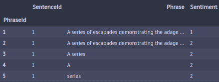
You can also get the information about the dataset via
train_data.info()
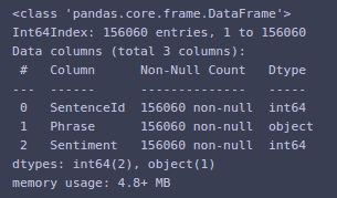
Here you can see that there are around 150k phrases each having a sentiment and a SentenceId.
You can see the sentiment distribution via
train_data['Sentiment'].value_counts()
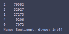
You will import some plotting libraries too so that you can do some basic visualization to get a better understanding of the dataset.
import matplotlib.pyplot as plt
import seaborn as sns
import pylab as pl
Before doing that, you will add a new column to the dataset, that is the length column. In this column, you will add the length of each phrase. This is going to add some extra information and help with plotting. You can add a new column in pandas via the following code. Notice what was used to apply with a built-in function len.
train_data['Length'] = train_data['Phrase'].apply(len)
We can now see the histogram of the length of the phrase via
train_data['Length'].plot(kind = 'hist' , bins = 50) 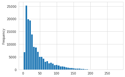
Next, you plot the histogram of the length of phrase via each sentiment by
ax = train_data.hist(column = 'Length', by = 'Sentiment', bins = 50 , figsize = (10,10));
pl.suptitle('Length via each Sentiment') 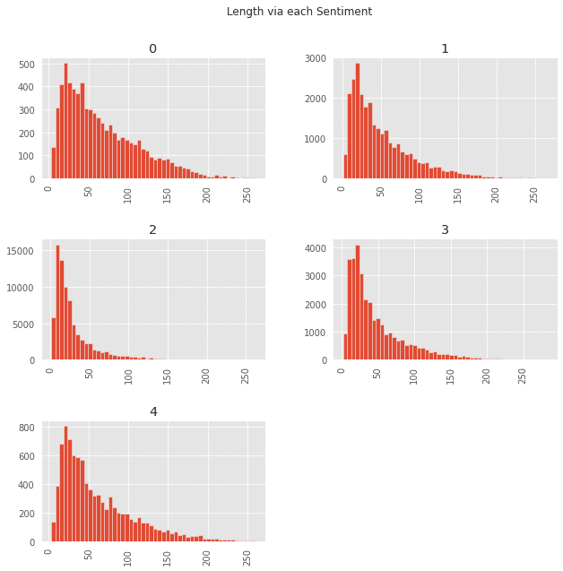
From these plots you can see that there are a lot of negative, and positive reviews that have lengths greater than 100. This tells us that if a customer is happy, or sad, they tend to write longer reviews compared to someone neutral.
You will write separate functions for each of the steps, and then combine those in a single cleaning function in order to understand the code easily, and call it in our pipeline later. A pipeline is used because any textual data used to test the model needs to be preprocessed the same way that the model is preprocessed, and it is difficult to call these functions explicitly. So by using a pipeline, you can combine them to simplify the task.
Tokenization
Tokenization is a way to split the strings into a list of words. In this example you’ll use the Natural Language Toolkit which has built-in functions for tokenization. There are 2 types of tokenization. The first type allows you to convert the whole sentence into a list, and the other type is where you can convert separate words into tokens.
def sentence_tokenize(text):
    """
    take string input and return a list of sentences.
    use nltk.sent_tokenize() to split the sentences.
    """
    return nltk.sent_tokenize(text):
def word_tokenize(text):
"""
:param text:
:return: list of words
"""
return nltk.word_tokenize(text) You can also use regex to tokenize it but it is a bit difficult. Though it gives you more control over your text. You can look up the detailed documentation on regular expressions here.
Now, to confirm it’s working, simply by calling it on our Phrase column.
train_data['Phrase'].apply(sentence_tokenize) And you can see the returned output
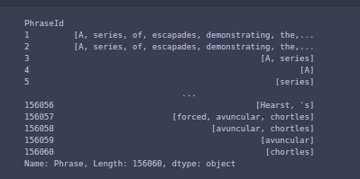
Now the next step is that you have to make sure that every letter is in lowercase so that the model will perform equivalently.
def to_lower(text):
        """
        :param text:
        :return:
            Converted text to lower case as in, converting "Hello" to "hello" or "HELLO" to "hello".
        """
        return text.lower()
We can confirm it via calling this function on our series
train_data['Phrase'].apply(lower_words) 
Here you can see a list of all the lowercase elements.
This is done not to assign to any variable, just to check whether the function is working correctly or not. It is a good practice to check individual functions before merging them into a pipeline.
Next, you will correct any misspellings in the list so that the model performs well because you should always practice the famous saying about machine learning models:
“Garbage in, Garbage Out”
So you have to make sure not to feed any garbage to the model. We can autocorrect the spellings via Speller from AutoCorrect. The one drawback is that it is really slow, and might take up to an hour or two for correcting the spelling on your dataset based on your CPU speed. So if you have a slow PC, you can ignore this step.
def autospell(text):
        """
        correct the spelling of the word.
        """
        spells = [spell(w) for w in (nltk.word_tokenize(text))]
        return " ".join(spells)
Here you pass in the text as an argument and apply an English Speller on that text to correct its spelling.
You can confirm it’s working by applying it to the first 200 rows.
train_data['Phrase'][:200].apply(autospell) 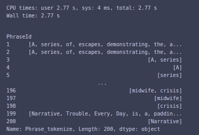
This has corrected the spelling for the first 200 rows.
The next thing we have to do is to remove the numbers. The main reason for removing the numbers is because typically numbers don’t contain much information. In some datasets, they might have meaning, but in this particular dataset there isn’t a ton of numbers or punctuations, so it is better to remove the remaining ones. This can be done simply using isdigit() method on a string, which will tell if the character is a digit or not, and remove it.
def remove_numbers(text):
        """
        take string input and return a clean text without numbers.
        Use regex to discard the numbers.
        """
        output = ''.join(c for c in text if not c.isdigit())
        return output
Now you can confirm it works by checking it on dummy data.
z = pd.Series(['a1', 'b2e', 'a3'])
z.apply(remove_numbers) 
You can check in the output that you have successfully removed the numbers.
Another important thing is to remove the punctuation, as they often do not carry any meaning to the sentiment analysis.
def remove_punct(text):

        return ''.join(c for c in text if c not in punctuation)
You have already imported the punctuation list from the String package and now you will just check if the sentence has those punctuations, and simply remove it.
The next step in cleaning the dataset is to remove the stopwords. Stopwords are those irrelevant words, which do not contain much meaning and do not help much in sentiment analysis.
Some of the stopwords are
You can remove them by using stopwords in nltk. Since they are already imported you can simply instantiate them, and use them to remove the stopwords.
def remove_stopwords(sentence):
        """
        removes all the stop words like "is,the,a, etc."
        """
        stop_words = stopwords.words('english')
        return ' '.join([w for w in nltk.word_tokenize(sentence) if not w in stop_words])
Next, you tokenize the sentence, and then simply add all the parts which are not in the stopwords list.
To check the output on 2 rows, you can call this function to make sure it is working correctly.
print(train_data['Phrase'][9:11])
train_data['Phrase'][9:11].apply(remove_stopwords) 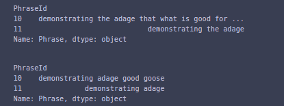
Normalization:
The last step for our data preprocessing is normalization. There are 2 common and famous techniques for Normalization. Those are stemming and lemmatization. In the English language, a single word can take many forms as per the usage, such as assign, assigns, assigned, assigning, etc. When you tokenize them, they refer to different words, but you know that all of these share a common meaning.
Stemming refers to the process of normalization, where we reduce a word to its base stem, for example, “automate”, “automatic”, “automation,” “automations” will be reduced to “automat” such that all these forms refer to automat.
Lemmatization on the other hand usually refers to doing things properly with the use of a vocabulary and morphological analysis, normally aiming to remove inflectional endings only and to return the dictionary form of a word.
Since Lemmatization returns the dictionary or lemma format and contains more meaning, this is the method chosen for this use case.
def lemmatize(text):
          wordnet_lemmatizer = WordNetLemmatizer()

        lemmatized_word = [wordnet_lemmatizer.lemmatize(word)for word in nltk.word_tokenize(text)]
        return " ".join(lemmatized_word)
Here you’ll tokenize the sentence, and call the lemmatizer on individual words of that tokenized list, and combine the lemmatized words.
This completes all the important data cleaning functions. Now you will combine them into a single function so that you can call that single function in our pipeline.
def preprocess(text):
        lower_text = to_lower(text)
        sentence_tokens = sentence_tokenize(lower_text)
        word_list = []
        for each_sent in sentence_tokens:
            lemmatizzed_sent = lemmatize(each_sent)
            clean_text = remove_numbers(lemmatizzed_sent)
            clean_text = remove_punct(clean_text)
            clean_text = remove_stopwords(clean_text)
            word_tokens = word_tokenize(clean_text)
            for i in word_tokens:
                word_list.append(i)
        return word_list
You can now check this function by calling it on some data to see if it is working fine, then use it on the whole dataset.
sample_data = train_data['Phrase'].head(5)
print(sample_data)
sample_data.apply(preprocess)
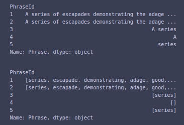
You can now see that the function is successfully cleaning the data.
Now that the “cleaning” of the dataset is complete, it’s time to transform it into a shape so that the machine learning model can understand it. Now, of course, a machine learning model does not understand textual data. It needs some numerical data to be fed into it so that it can perform the computations.
You can use two main tools.
- CountVectorizer
- TF-IDF
CountVectorizer is a great feature extraction tool provided by sklearn. The basic purpose of CountVectorizer is that it converts a given text into a vector-based on the count (frequency) of the occurrence of each word in a list. It creates a sparse matrix of the count of the numbers.
You can import it via
from sklearn.feature_extraction.text import CountVectorizer Now you’ll need to get the whole data into the CountVectorizer’s sparse matrix. But before you feed that, you’ll have to pass the whole dataset through the preprocessing function. CountVectorizer gives us this option.
You can do it by passing the preprocessing function to the analyzer argument when creating the object.
bow = CountVectorizer(analyzer=preprocess) The next thing is TF-IDF also known as term-frequency times inverse document-frequency. TF means term frequency, which refers to the frequency of appearance of a word divided by the total number of words in the document.
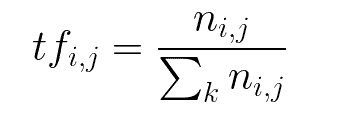
IDF means inverse document frequency which is computed via a log of the number of documents that contain the word ‘w’. It determines the weight of the rare words across all documents in the corpus.

TF-IDF is simply the product of Term Frequency and Inverse Document Frequency i.e

Instead of manually calculating the TF-IDF, it is built-into sklearn and you can just import it and use it.
from sklearn.feature_extraction.text import TfidfTransformer
tfidf = TfidfTransformer()
Machine Learning to predict Sentiments
The last thing to go over before combining all these things is the Machine Learning Algorithm that you are going to use. In this example, you’ll use the NaiveBayes Classifier. Naive Bayes tends to be the baseline model for every sentiment analysis task. You can find people using it in a lot of Kaggle competitions on sentiment analysis.
The way it works is that it finds out the probabilities of the classes assigned to the text by using the joint probabilities of words and classes. The equation for computing the probabilities is:

Given the feature vector (x1,…, xn) and the class Ck, Bayes theorem is stated mathematically having the following relationship.

Naïve Bayes only assumes one fact that one event in a class should be independent of another event belonging to the same class. The algorithm also assumes that the predictors have an equal effect on the outcomes or responses in the data.
There are several types of Naive Bayes which you can discover such as Gaussian Naive Bayes, Bernoulli Naive Bayes, Multinomial Naive Bayes, etc. This example is going to use Multinomial Naive Bayes.
Sklearn comes with Naive Bayes already implemented in it, making it the most convenient to use.
from sklearn.naive_bayes import MultinomialNB
classifier = MultinomialNB()
Now you are going to combine all these steps into a machine learning pipeline. The benefit of a pipeline is that you do not have to call all the data preprocessing and wrangling steps manually on new data, they are automatically called by the pipeline, and you just have to pass through the pipeline.
Sklearn has a very good pipeline class which will serve the job.
from sklearn.pipeline import Pipeline

pipeline = Pipeline([
    ('bow', bow),  # strings to token integer counts
    ('tfidf', tfidf),  # integer counts to weighted TF-IDF scores
    ('classifier', classifier),  # train on TF-IDF vectors w/ Naive Bayes classifier
])
Notice you are passing in the objects defined earlier, the bow is the CountVectorizer object that has a preprocess function as an analyzer, tfidf is our TF-IDF transformer object, and classifier is the recent object created for Naive Bayes classification.
Now, you’ll fit this pipeline on the training data and sentiments.
pipeline.fit(train_data['Phrase'],train_data['Sentiment']) This will train our model on the pipeline using the phrases and their sentiments as the outputs. We can find our accuracy by using the score function on the pipeline.
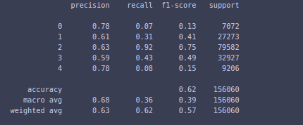
pipeline.score(train_data['Phrase'], train_data['Sentiment']) For a detailed evaluation of the model, you can see the classification report to get to know the accuracy, precision, and recall values.
from sklearn.metrics import classification_report

all_predictions = pipeline.predict(train_data['Phrase'])
print(classification_report(train_data['Sentiment'], all_predictions)) 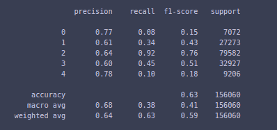
Here you can see the precision, recall, and f1-score for all classes. The model is more precise in predicting very negative(0) to very positive(4). Now, there are several ways to improve the model, including GridCVSearch, more focus on cleaning, changing the classifier, etc. but we are not going to put much focus on that. And in fact, it is a good accuracy for such a simple model.
Data Cleaning and Model prediction using SpaCy
Above NLTK is used to clean the data and preprocess it. Another tool that can be used is known as SpaCy. SpaCy is a library designed for fast and practical work, to avoid wasting time on NLP projects.
You can simply download this library from the command line using the following command.
pip install spacy You also need to download its English language model as we are working with the English Language.
python -m spacy download en The following example will use dummy data using spaCy and finally combine all these steps in the Movie Reviews dataset to predict the sentiment.
Now you have to import it and make the object for it.
import spacy
nlp = spacy.load('en')
Tokenization using spaCy
You can convert any text into a spaCy document with linguistic annotations, on which to perform some operations via
dummy_text = """Hopefully you are enjoying this tutorial and learning new things"""

my_doc = nlp(dummy_text)
Check the type of my_doc.
print(type(my_doc)) Now simply word tokenize the dataset, by importing the Tokenizer package from spaCy.
from spacy.tokenizer import Tokenizer
tokenizer = Tokenizer(nlp.vocab)
Pass the text to our tokenizer object.
tokens = tokenizer(my_doc.text) To see these tokens you can use:
list(tokens) Removing stop words
Removing stop words is also very easy using spaCy. You can import the stop words from the stop_words class that is built into spaCy.
from spacy.lang.en.stop_words import STOP_WORDS
From here, you can see all the stop words that are in spaCy by printing it
print('First twenty stop words: %s' % list(STOP_WORDS)[:20])
Now spaCy includes some of the useful token attributes, one of which is is_sent which returns True if the word is a stopword, and false in the other case.
You will simply loop over the my_doc and append all the non-stop words into our output list.
filtered_sent=[]
for word in my_doc:
    if word.is_stop==False:
        filtered_sent.append(word)
print("Filtered Sentence:",filtered_sent)
The stop words have been removed.
Lemmatization
Spacy includes a built-in attribute lemma_ to reduce a word to its lemma form. You can see the lemma form of each word in the doc via
for i in my_doc:
print("Original Word, ", i, " Lemma form, ", i.lemma_) 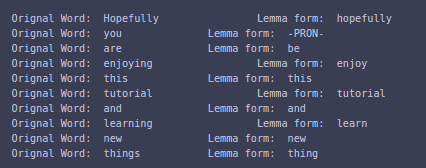
Here, it is showing the reduced form of every word. Notice where it says -PRON- here which means that it is a pronoun, and can not be reduced to any other format.
Removing Punctuation
Let’s take a look at another example, which contains some punctuation.
my_doc = nlp("I am learning well, and progressing good!") SpaCy provides a Part of Speech attribute pos_ which tells you the respective part of speech of that word.
for word in my_doc:
print(word.text,word.pos_) 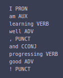
This tells you all the parts of speech of every single word. You can remove the punctuations by comparing the part of speech to PUNCT.
nopunc = []
for word in my_doc:
    if word.pos_ != 'PUNCT':
        nopunc.append(word)
print(nopunc)
Here, you can see that all the punctuation has been successfully removed.
Now that you’ve seen the important elements of spaCy, you will create a preprocess function that will contain all the important parts.
import string # for punctuations
from spacy.lang.en.stop_words import STOP_WORDS  # removing stopwords


punctuations = string.punctuation

nlp = spacy.load('en') #english model for spacy
stop_words = spacy.lang.en.stop_words.STOP_WORDS #stop words


def preprocess(text):
    #removing the digits
    nonum = ''.join([i for i in text if not i.isdigit()])
    # Creating our token object, which is used to create documents with linguistic annotations.
    tokenized_list = nlp(nonum)

    # Lemmatizing each token and converting each token into lowercase
    tokenized_list = [ word.lemma_.lower().strip() if word.lemma_ != "-PRON-" else word.lower_ for word in tokenized_list ]

    # Removing stop words
    tokenized_list = [ word for word in tokenized_list if word not in stop_words and word not in punctuations ]

    # return a preprocessed list of tokens
    return tokenized_list
This function does a complete job of cleaning the data. You can test it via
preprocess("Hello1 ! I am a good boy") Since you are now done with data preprocessing, the next step is going to be generating a sparse matrix using CountVectorizer and then TF-IDF using sklearn.
Notice the use of sklearn.feature_extraction.text.TfidfTransformer which only converts a sparse matrix to its tf-idf format. In this case, you are going to use sklearn.feature_extraction.text.TfidfVectorizer which has CountVectorizer included in it so we do not have to use it as a separate step
from sklearn.feature_extraction.text import TfidfVectorizer
from sklearn.linear_model import MultinomialNB
from sklearn.pipeline import Pipeline

classifier = MultinomialNB()
tfidf_vector = TfidfVectorizer(tokenizer = preprocess)
# Create pipeline
pipe = Pipeline([('tfidf',tfidf_vector),
                 ('classifier', classifier)])

# model generation
pipe.fit(train_data['Phrase'],train_data['Sentiment'])
We can check the accuracy of the data by calling the score method.
pipe.score(train_data['Phrase'],train_data['Sentiment']) To evaluate it further you can use the data via classification report.
from sklearn.metrics import classification_report
Pred = pipe.predict(train_data['Phrase'])
print(classification_report(train_data['Sentiment'], Pred))
Note that there is a separate test file in the kaggle directory, which you can download to further analyze your model.
Building Your Own NLP Sentiment Analyzer using PyTorch
Until now, we’ve looked at traditional machine learning algorithms, which have a drawback when dealing with sequential data. This drawback is covered by LSTMs and RNN which are very good in sequential data. You can learn more about LSTMs and Sequential Data in the article “PyTorch LSTM: The definitive Guide” which covers issues with traditional neural networks and how LSTMs and RNNs solve these problems.
If you do not have previous knowledge about LSTMs and RNNs, you might want to go over the article above.
So far you’ve seen the two important techniques of converting words to vectors are CountVectorizer and TF-IDF. Some of the more advanced techniques are
- Word2Vec
- Glove
- Simple Embedding Layer etc.
These are techniques that are unsupervised learning techniques. These help us learn representation for text where words that have the same meaning have a similar representation. There are pre-trained word embeddings also available which can be used in your models.
This example will use the IMDB movie reviews dataset which you can download from kaggle here. This dataset has 50k reviews of movies and has binary sentiments i.e Positive or Negative.
First you’ll import the important libraries..
import numpy as np # linear algebra
import pandas as pd # data processing, CSV file I/O (e.g. pd.read_csv)
import torch #pytorch
import torch.nn as nn #for our model class
import torch.nn.functional as F
from nltk.corpus import stopwords #removing stop words
from collections import Counter #counting the unique numbers
import string
import re #regex
import seaborn as sns #plotting
import matplotlib.pyplot as plt #plotting
from torch.utils.data import TensorDataset, DataLoader #data prep
from sklearn.model_selection import train_test_split #splitting the dataset for training and testing
You can check if you have a GPU or not using PyTorch, and enable it.
is_cuda = torch.cuda.is_available()

# If we have a GPU available, we'll set our device to GPU. We'll use this device variable later in our code.
if is_cuda:
    device = torch.device("cuda")
    print("GPU is available")
else:
    device = torch.device("cpu")
    print("GPU not available, CPU used")
The next step is loading the dataset after downloading it.
df = pd.read_csv('IMDB Dataset.csv')
df.head()
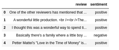
You can see the head that is
Now the next important step is to split the data set into 2 portions for training and testing.
X,y = df['review'].values,df['sentiment'].values
x_train,x_test,y_train,y_test = train_test_split(X,y,stratify=y)
print(f'shape of train data is {x_train.shape}')
print(f'shape of test data is {x_test.shape}')
Since you have used the stratify=y argument, there is an equal number of positive and negative examples in the training and testing datasets. This can be confirmed by plotting the number of classes using Seaborn.
dd = pd.Series(y_train).value_counts()
sns.barplot(x=np.array(['negative','positive']),y=dd.values)
plt.show()

The next step is to preprocess the data. This time you will use regular expressions mostly. Most people think that regex is hard, but if you understand the basics of it, they become straightforward. You can take a look at this tutorial if you are unaware of regex.
def preprocess_string(s):
    # Remove all non-word characters
    s = re.sub(r"[^\w\s]", '', s)
    # Replace all runs of whitespaces with no space
    s = re.sub(r"\s+", '', s)
    # replace digits with no space
    s = re.sub(r"\d", '', s)

    return s
The next step is tokenization.
def tockenize(x_train,y_train,x_val,y_val):
    word_list = []

    stop_words = set(stopwords.words('english')) #for removing stop words
    for sent in x_train:
        for word in sent.lower().split(): #lower case sentence splitted in list
            word = preprocess_string(word) #preprocess that word using the above function
            if word not in stop_words and word != '':
                word_list.append(word) #if not stop word then append

    corpus = Counter(word_list) #counting the words occurence
    # sorting on the basis of most common words
    corpus_ = sorted(corpus,key=corpus.get,reverse=True)[:1000]
    # creating a dict
    onehot_dict = {w:i+1 for i,w in enumerate(corpus_)} #this will create a dictionary with their numbers based on most common words

    # tockenize
    final_list_train,final_list_test = [],[]
    for sent in x_train:
            final_list_train.append([onehot_dict[preprocess_string(word)] for word in sent.lower().split if preprocess_string(word) in onehot_dict.keys()]) #picking the number of the word after preprocessing it
    for sent in x_val:
            final_list_test.append([onehot_dict[preprocess_string(word)] for word in sent.lower().split if preprocess_string(word) in onehot_dict.keys()]) #picking the number of the word after preprocessing it

    encoded_train = [1 if label =='positive' else 0 for label in y_train] #encoding the labels
    encoded_test = [1 if label =='positive' else 0 for label in y_val]
    return np.array(final_list_train), np.array(encoded_train), np.array(final_list_test), np.array(encoded_test),onehot_dict #returning these 4 values
Now you just need to call this function to the data.
x_train,y_train,x_test,y_test,vocab = tockenize(x_train,y_train,x_test,y_test) You can check the dictionary or vocabulary length via
print(f'Length of vocabulary is {len(vocab)}') Next, you will analyze the length of the sequences so that you can padd them.
rev_len = [len(i) for i in x_train]
pd.Series(rev_len).hist()
plt.show()
pd.Series(rev_len).describe() 
Here you can see most of the reviews lie between 0 to 100. Some of them lie in the 200-400 range.
Next is Padding. Since the reviews are not of the same length you’ll need to pad the sequences. Different research papers have suggested that padding 0s to the sequence has improved the performance of the model a lot.
In-order to make sure that no important information is missed out, you can padd the sequences to the maximum sequence length which is nearly 400 to 500 as shown in the graph.
def padding_(sentences, seq_len):
    features = np.zeros((len(sentences), seq_len),dtype=int)
    for ii, review in enumerate(sentences):
        if len(review) != 0:
            features[ii, -len(review):] = np.array(review)[:seq_len]
    return features
#we have very less number of reviews with length > 500.
x_train_pad = padding_(x_train,500)
x_test_pad = padding_(x_test,500) Next thing is to create our dataset as Tensors from Numpy arrays. You will also shuffle the dataset. You will use TensorDataset from torch.util.data to make these in Tensor format.
# create Tensor datasets
train_data = TensorDataset(torch.from_numpy(x_train_pad), torch.from_numpy(y_train))
valid_data = TensorDataset(torch.from_numpy(x_test_pad), torch.from_numpy(y_test))

# batch size
batch_size = 50

#shuffling
train_loader = DataLoader(train_data, shuffle=True, batch_size=batch_size)
valid_loader = DataLoader(valid_data, shuffle=True, batch_size=batch_size)
To define the LSTM model with word embeddings, you are going to use a simple Word Embedding layer, but you can use pre-trained layers to further improve the model results.
Now it’s time to design the model. Remember that a PyTorch model is inherited from the base class torch.nn.Module which has already been imported. Let’s separately go over the functions of the class, and then combine them all into a code block.
class SentimentRNN(nn.Module): #class name
    def __init__(self,no_layers,vocab_size,hidden_dim,embedding_dim,drop_prob=0.5):
        super(SentimentRNN,self).__init__() #initializing base class

        self.output_dim = output_dim #output dimensions
        self.hidden_dim = hidden_dim #hidden dimensions

        self.no_layers = no_layers #number of layers
        self.vocab_size = vocab_size #vocabulary size

        # embedding
        self.embedding = nn.Embedding(vocab_size, embedding_dim) #embedding of vocabulary size and embedding dimensions

        #lstm
        self.lstm = nn.LSTM(input_size=embedding_dim,hidden_size=self.hidden_dim,
                           num_layers=no_layers, batch_first=True)


        # dropout layer
        self.dropout = nn.Dropout(0.4)

        # linear and sigmoid layer
        self.fc0 = nn.Linear(self.hidden_dim, 512) #first drop out
        self.fc1 = nn.Linear(512, 256) #1st fc layer
        self.dropout1 = nn.Dropout(0.2) #2nd drop out
        self.fc = nn.Linear(256, output_dim) #2nd fully connected layer
        self.sig = nn.Sigmoid() #for last layer
Here all the layers that will be used have been defined. There is an embedding layer, 1 LSTM layer that will be stacked i.e hidden layers of LSTM. Then there are some dropout layers and 2 fully connected layers with some neurons.
The next thing to define in the class is the forward pass. You will also define another function in the class named forward in which you will define the forward pass.
def forward(self,x,hidden):
        batch_size = x.size(0) #fetching batch size
        # embeddings and lstm_out
        embeds = self.embedding(x)  # shape: Batch x S x Feature   since batch = True
        lstm_out, hidden = self.lstm(embeds, hidden) #passing our embedded layer into lstm

        lstm_out = lstm_out.contiguous().view(-1, self.hidden_dim)  #reshaping the lstm output

        # dropout and fully connected layer
        out = self.dropout(lstm_out)
        out = self.fc0(out)
        out = self.dropout1(out)
        out = self.fc1(out)
        out = self.fc(out)

        # sigmoid function for binary classification output
        sig_out = self.sig(out)

        # reshape to be batch_size first
        sig_out = sig_out.view(batch_size, -1)

        sig_out = sig_out[:, -1] # get last batch of labels

        # return last sigmoid output and hidden state
        return sig_out, hidden
Here you have passed the input into the word embedding, and then passed the previous hidden state and the word embedding inside LSTM layers (notice that there can be many hidden layers in our LSTM). Then you reshape the output so that you can pass it to the fully connected layers. You’ll then apply the layers and dropouts step by step. In the end you will use Sigmoid activation function because it is a binary classification problem (0 or 1). You will return the hidden state and final sigmoid layer output.
The next step is initializing the hidden state. You could ignore it, but it will affect the performance. You can learn more about it in the PyTorch official discussion here where Soumith Chintala the creator of PyTorch discusses this issue. Moreover, you can refer to StackOverflow for this problem where it is discussed by the people.
def init_hidden(self, batch_size):
        ''' Initializes hidden state '''
        # Create two new tensors with sizes n_layers x batch_size x hidden_dim,
        # initialized to zero, for hidden state and cell state of LSTM using torch.zeros
        h0 = torch.zeros((self.no_layers,batch_size,self.hidden_dim)).to(device)
        c0 = torch.zeros((self.no_layers,batch_size,self.hidden_dim)).to(device)
        hidden = (h0,c0)
        return hidden
The combined code for the model is
class SentimentRNN(nn.Module):
    def __init__(self,no_layers,vocab_size,hidden_dim,embedding_dim,drop_prob=0.5):
        super(SentimentRNN,self).__init__()

        self.output_dim = output_dim #output dimensions
        self.hidden_dim = hidden_dim #hidden dimensions

        self.no_layers = no_layers #number of layers
        self.vocab_size = vocab_size #vocabulary size

        # embedding
        self.embedding = nn.Embedding(vocab_size, embedding_dim) #embedding of vocabulary size and embedding dimensions
        #lstm
        self.lstm = nn.LSTM(input_size=embedding_dim,hidden_size=self.hidden_dim,
                           num_layers=no_layers, batch_first=True)

        # dropout layer
        self.dropout = nn.Dropout(0.4)

        # linear and sigmoid layer
        self.fc0 = nn.Linear(self.hidden_dim, 512) #first drop out
        self.fc1 = nn.Linear(512, 256) #1st fc layer
        self.dropout1 = nn.Dropout(0.2) #2nd drop out
        self.fc = nn.Linear(256, output_dim) #2nd fully connected layer
        self.sig = nn.Sigmoid() #for last layer

    def forward(self,x,hidden):
        batch_size = x.size(0)
        # embeddings and lstm_out
        embeds = self.embedding(x)  # shape: B x S x Feature   since batch = True
        #print(embeds.shape)  #[50, 500, 1000]
        lstm_out, hidden = self.lstm(embeds, hidden)

        lstm_out = lstm_out.contiguous().view(-1, self.hidden_dim)

        # dropout and fully connected layer
        out = self.dropout(lstm_out)
        out = self.fc0(out)
        out = self.dropout1(out)
        out = self.fc1(out)
        out = self.fc(out)

        # sigmoid function
        sig_out = self.sig(out)

        # reshape to be batch_size first
        sig_out = sig_out.view(batch_size, -1)

        sig_out = sig_out[:, -1] # get last batch of labels

        # return last sigmoid output and hidden state
        return sig_out, hidden


    def init_hidden(self, batch_size):
        ''' Initializes hidden state '''
        # Create two new tensors with sizes n_layers x batch_size x hidden_dim,
        # initialized to zero, for hidden state and cell state of LSTM
        h0 = torch.zeros((self.no_layers,batch_size,self.hidden_dim)).to(device)
        c0 = torch.zeros((self.no_layers,batch_size,self.hidden_dim)).to(device)
        hidden = (h0,c0)
        return hidden
Next, you will define some parameters needed for the model.
no_layers = 4 #4 hidden LSTM stacked layers
vocab_size = len(vocab) + 1 #extra 1 for padding
embedding_dim = 64 # embedding dimensions
output_dim = 1 #single output 1 or 0
hidden_dim = 256 # hidden dimensions
model = SentimentRNN(no_layers,vocab_size,hidden_dim,embedding_dim,drop_prob=0.5)
#moving to gpu if available
model.to(device)
You can see the model details by printing the models.
print(model) 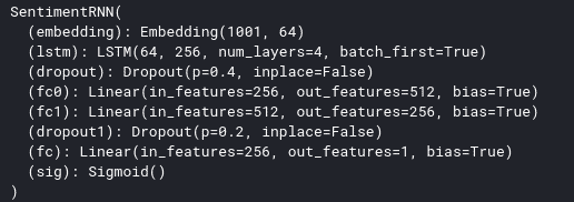
Now you will define a function for accuracy.
def acc(pred,label):
    pred = torch.round(pred.squeeze()) #remove extra dimensions
    return torch.sum(pred == label.squeeze()).item()  #correct predictions vs label
Next, define some hyperparameters for the model.
lr=0.001 #learning rate
criterion = nn.BCELoss() #binary cross entropy for binary classification
optimizer = torch.optim.Adam(model.parameters(), lr=lr) #adam optimizer
Next, you’ll define some more variables, which will be used later.
clip = 5 #gradient clipping for exploding gradients
epochs = 10 #number of epochs
valid_loss_min = np.Inf #setting loss for minimum i.e infinity epochs
# train for some number of epochs
epoch_tr_loss,epoch_vl_loss = [],[]  #lists for appending per epochs statistics to visualize
epoch_tr_acc,epoch_v_acc = [],[]
You will complete forward pass by looping through the dataset for the number of epochs previously defined, calling the forward() function, append the metrics in the list, compute the loss, backpropagate and improve the performance via Adam optimizer, and calculate the accuracy. You’ll perform the same on the validation set except for the backpropagation and improving the score as validation sets are used to measure the performance of the model, not to train them.
for epoch in range(epochs):
    train_losses = []
    train_acc = 0.0
    model.train()
    # initialize hidden state
    h = model.init_hidden(batch_size)
    for inputs, labels in train_loader: #training data

        inputs, labels = inputs.to(device), labels.to(device)
        # Creating new variables for the hidden state, otherwise
        # we'd backprop through the entire training history
        h = tuple([each.data for each in h])

        model.zero_grad() #zero gradients before starting the training
        output,h = model(inputs,h) #forward pass

        # calculate the loss and perform backprop
        loss = criterion(output.squeeze(), labels.float()) #criterion loss
        loss.backward() # computes loss
        train_losses.append(loss.item()) #appending the loss
        # calculating accuracy
        accuracy = acc(output,labels)
        train_acc += accuracy

        #`clip_grad_norm` helps prevent the exploding gradient problem in RNNs / LSTMs.
        nn.utils.clip_grad_norm_(model.parameters(), clip)
        optimizer.step() #improving the loss via optimizer using back prop (ADAM optimizer)


    val_h = model.init_hidden(batch_size) #initialize the hidden state
    val_losses = []
    val_acc = 0.0
    model.eval()
    for inputs, labels in valid_loader: #validation data
            val_h = tuple([each.data for each in val_h]) #separate variable for hidden state

            inputs, labels = inputs.to(device), labels.to(device) #checking if gpu or not

            output, val_h = model(inputs, val_h) #forward pass
            val_loss = criterion(output.squeeze(), labels.float()) # loss

            val_losses.append(val_loss.item()) #appending loss

            accuracy = acc(output,labels)
            val_acc += accuracy

    epoch_train_loss = np.mean(train_losses)  #mean of the loss for calculating epoch loss
    epoch_val_loss = np.mean(val_losses) #same for validation loss
    epoch_train_acc = train_acc/len(train_loader.dataset) #acc for epoch
    epoch_val_acc = val_acc/len(valid_loader.dataset) #vali acc for epoch
    epoch_tr_loss.append(epoch_train_loss)
    epoch_vl_loss.append(epoch_val_loss)
    epoch_tr_acc.append(epoch_train_acc)
    epoch_vl_acc.append(epoch_val_acc)
    print(f'Epoch {epoch+1}')
    print(f'train_loss : {epoch_train_loss} val_loss : {epoch_val_loss}')
    print(f'train_accuracy : {epoch_train_acc*100} val_accuracy : {epoch_val_acc*100}')
    if epoch_val_loss <= valid_loss_min:
        torch.save(model.state_dict(), '../working/state_dict.pt') #saving the model in dictionary in .pt format
        print('Validation loss decreased ({:.6f} --> {:.6f}).  Saving model ...'.format(valid_loss_min,epoch_val_loss))
        valid_loss_min = epoch_val_loss
    print(25*'==') #for epoch ending symbol
Comments have been added to the code, which you can understand by reading the code carefully.
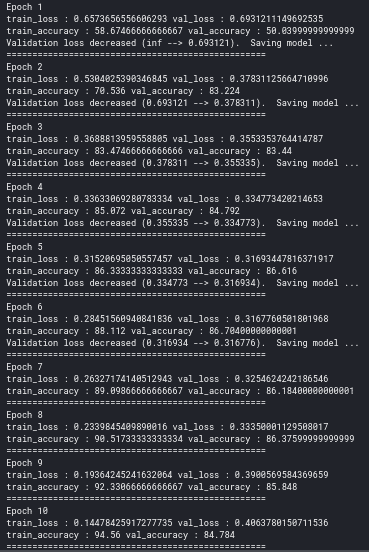
You can plot the model statistics by using the lists in which you appended the accuracy and loss of the model.
fig = plt.figure(figsize = (20, 6))
plt.subplot(1, 2, 1)
plt.plot(epoch_tr_acc, label='Train Acc') #training list
plt.plot(epoch_vl_acc, label='Validation Acc') #validation list
plt.title("Accuracy")
plt.legend()
plt.subplot(1, 2, 2)
plt.plot(epoch_tr_loss, label='Train loss') #training loss
plt.plot(epoch_vl_loss, label='Validation loss') #validation loss
plt.title("Loss")
plt.legend()
plt.grid() #grid
plt.show() #showing the plots

You can see that our model is overfitting, and can be fixed by regularization, dropout or batch normalization, etc.
You can create a function to test our model.
def predict_text(text):
        word_seq = np.array([vocab[preprocess_string(word)] for word in text.split()
                         if preprocess_string(word) in vocab.keys()]) #preprocess data
        word_seq = np.expand_dims(word_seq,axis=0) #expanding the dimensions for lstm
        pad =  torch.from_numpy(padding_(word_seq,500)) #padding the sequences
        inputs = pad.to(device) #checking if gpu or not
        batch_size = 1 #batch size 1 for 1 input at 1 time
        h = model.init_hidden(batch_size) #initializing the hidden state
        h = tuple([each.data for each in h]) # hidden state variable
        output, h = model(inputs, h) #forward pass through the model
        return(output.item()) #returning the output from sigmoid
Now check any random review to compare our results.
import random
index = random.randint(0,25000)
print(df['review'][index])
print(80*'=')
print("Actuall Sentiment is ", df['sentiment'][index])
pro = predict_text(df['review'][index])
sent = 'positive' if pro >=0.5 else 'negative'
print("Predicted Sentiment is ", sent, " with a probability of ", pro) 
Here you can see that the model is performing pretty well on the dataset.
You can improve this mode via
- Regularization
- Hyperparameter Tuning
- Adding more layers
- Using Bi-Directional LSTMS
- Using Pre-trained Word Embeddings such as Glove or Word2Vec etc.
Next Steps with Sentiment Analysis
- Kaggle often announces new Sentiment Analysis Competitions, so you can try one of them.
- Deploying Sentiment Analysis through Kubernetes.
- Real-time Sentiment Analysis
- Intent Analysis
- Deploying a Sentiment Analysis application through Flask or Django
- Using Transformers, BERT, GPT, or other related high performing NLP models.
References:


