
The process of optimizing the hyper-parameters of a machine learning model is known as hyperparameter tuning. This process is crucial in machine learning because it enables the development of the most optimal model. Therefore, an ML Engineer has to try out different parameters and settle on the ones that provide the best results for the problem they are solving. The best hyper-parameters are the ones that result in the least error in the validation set.
In this article, we will look at various tools and strategies that you can start using today in your machine learning workflow.
Let’s get to it.
What's a hyperparameter?
Hyper-parameters are parameters of an algorithm that determine the performance of that model. The process of tuning these parameters in order to get the most optimal parameters is known as hyper-parameter tuning. The best parameters are the parameters that result in the best accuracy and or the least error. Let’s take an example where you are defining the parameters of a `GradientBoostingRegressor`:
parameters = {
    'loss': ['ls', 'lad','huber','quantile'],
    'learning_rate': [0.1, 0.2,0.3],
    'max_depth': [3,5,6]
}
The loss,learning rate and maximum depth are parameters that can be tuned:
- the loss is the loss function that will be used in the boosting process
- the learning rate is a multiplicative factor that is used for the leave values, and
- the `max_depth` is the maximum depth for each tree
It is important to note that hyperparameters are different from model parameters. Model parameters are learned during the process of training a machine learning model. For example, in a ridge regression model, the coefficients are learned during the training process. The hyperparameters are the parameters that determine the best coefficients to solve the regression problem.
It is not possible to mention all the hyper-parameters for all the models. However, for example when working with Scikit-learn, one can always refer to the documentation of the algorithm for parameters that can be tuned.
Hyperparameter types
The hyper-parameters to tune can be of various types. Usually, the documentation of the algorithm you are working on will dictate the data type of the parameter to be passed. Passing the wrong type will usually result in an error. For example, let’s look at the parameters defined above:
- the loss is a categorical type,
- the learning rate is a float, and
- the maximum depth is an integer
When passing these parameters, ensure you refer to the documentation of the algorithm you are using. This will guarantee that you don’t get type errors while optimizing your model.
How hyperparameter tuning works
Given a set of parameters, hyper-parameter tuning works by identifying the set of parameters that result in the highest accuracy and or least error. This is done by running multiple trials with various combinations of hyper-parameters. In this process the results are tracked so that the parameters which result in the best performance are settled on.
What hyperparameter tuning optimizes
Hyper-parameter tuning works by either maximizing or minimizing the specified metric. For example, you will usually try to maximize the accuracy while trying to reduce the loss function. These metrics are computed from various iterations of different sets of hyper-parameters.
Methodologies of Hyperparameter Tuning
There are several ways that you can tune your parameters. Let’s look at them in this section.
Grid Search
In Grid Search, parameters are defined and searched exhaustively. Since a model is built for all possible combinations of parameters, this process can be computationally expensive and time consuming. In Scikit-learn this can be implemented using the `GridSearchCV` module. Let’s take a look at how to perform grid search using the parameters defined at the beginning of this piece.
Start by creating a simple regression dataset and then split it into a training and testing set.
from sklearn.datasets import make_regression
X, y = make_regression(n_samples=10000, n_features=12, n_informative=10,  random_state=42)
from sklearn.model_selection import train_test_split
X_train, X_test, y_train, y_test = train_test_split(X, y, test_size=0.30, random_state=42)
Next, define the parameters that will be searched (These parameters have already explained).
parameters = {
    'loss': ['ls', 'lad','huber','quantile'],
    'learning_rate': [0.1, 0.2,0.3],
    'max_depth': [3,5,6]
}
Next use the `GradientBoostingRegressor` for this example. Let’s import it.
from sklearn.ensemble import GradientBoostingRegressor You also need to import the `GridSearchCV` module.
import the from sklearn.model_selection import GridSearchCV The next step is to perform the search using `GridSearchCV`. As you do so, you have to pass the estimator, parameters and the cross validation strategy you would like to use. There are a couple of options for the cross validation:
- when nothing is passed, the default 5-fold cross validation will be used
- passing an integer indicates that you are specifying the number of folds in a (Stratified)KFold
Specifying `verbose=1` just prints the progress and performance. Since this will be a resource intensive process passing `n_jobs=-1` will make use of all the available CPUs. This ensures that the search for the best parameters runs in parallel.
regressor = GridSearchCV(GradientBoostingRegressor(), parameters, verbose=1,cv=5,n_jobs=-1)
regressor.fit(X_train,y_train)
A hyper-parameter of `GridSearchCV` known as `refit` is set to True by default. The purpose of this is to retrain the regressor on the optimal parameters that will be obtained. Therefore, once the search is done, we will have a regressor that is ready for use.
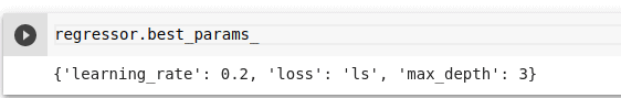
When the process is done, the best parameters can be obtained via the `best_params_` attribute.
regressor.best_params_
All the cv results can be seen via the `cv_results_` attribute.
regressor.cv_results_ You can also take a look at the best estimator and its parameters.
regressor.best_estimator_ 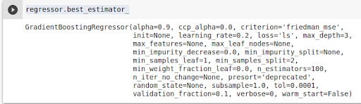
Since `refit` was true, you can run predictions on the estimator immediately.
predictions = regressor.predict(X_test) You can also obtain the test results.
from sklearn.metrics import mean_absolute_error, mean_squared_error
import numpy as np

print('Root Mean Squared Error is {} '.format(np.sqrt(mean_squared_error(y_test,
                                                    regressor.predict(X_test)))) )
Random Search
In this method, a randomized search is performed over the parameters. In this case each configuration is sampled from a distribution over possible parameter values. Unlike `GridSearchCV`, not all the specified parameters will be tried. Compared to exhaustive search, this method is advantageous because you can choose the maximum number of trials wanted for this search. The parameters to be sampled are specified using a dictionary. For algorithms that take statistical distributions as parameters, the `scipy.stats` module can be used to pass them. Note that you can always get the parameters for a given estimator by using `estimator.get_params()`.
Sticking with that Gradient Boosting Regressor problem, you can define the distribution to be sampled as follows:
distributions = dict(max_depth=[3,5,6],learning_rate= [0.1, 0.2,0.3], loss = ['ls', 'lad','huber','quantile'])
Next import `RandomizedSearchCV` and fit it onto the training set. Apart from the `n_iter` parameter all the other parameters are similar to the `GridSearchV` parameters. The `n_iter` parameter dictates the number of parameters settings that will be sampled. This means that when this number is reached then the process will stop whether or not other setting combinations would have given better results. This method therefore trades off the run time to the quality of the solution.
from sklearn.model_selection import RandomizedSearchCV
regressor = RandomizedSearchCV(GradientBoostingRegressor(), distributions, verbose=1,cv=5,n_jobs=-1,n_iter=10)
regressor.fit(X_train,y_train)
Once this is done, the best parameters, the CV results and the best estimator can be obtained just like done previously. Also, since the `refit` parameter is true by default, the regressor is ready for use.
Bayesian optimization
In this method, the results obtained from one experiment can be used to improve sampling for the next experiment. This process is repeated until the most optimal parameters are obtained. The method is based on the Bayes Theorem. It is majorly used when the objective function in question is complex or computationally expensive to evaluate.
The Scikit-Optimize package is one package that enables the performance of Bayesian optimization. It is a tool that is built on top of Scipy, NumPy, and Scikit-Learn.
Like in Random Search, not all parameters are sampled. The maximum number of parameters are defined using the `n_iter` parameter. We can implement this search using the `BayesSearchCV` class. Ensure that Scikit-Optimize is installed.
The parameters to be passed to this class have to be of the `skopt.space.Dimension` instance. You’ll therefore start by importing those:
- `Real` indicates any real value. For this, you need to pass a lower bound and an upper bound and both are inclusive,
- `Categorical` indicates that the parameter is categorical, for example the loss function,
- `Integer` means that the parameter is an integer, for example the maximum depth
from skopt.space import Real, Categorical, Integer Let’s now import BayesSearchCV, pass the estimator and its parameters. The hyper-parameters are passed in as a dictionary. Since this class is a Scikit-learn wrapper, the other parameters such as `cv`,` verbose`, and `n_jobs` remain the same.
from skopt import BayesSearchCV
regressor = BayesSearchCV(
    GradientBoostingRegressor(),

     {
         'learning_rate': Real(0.1,0.3),
         'loss': Categorical(['lad','ls','huber','quantile']),
'max_depth': Integer(3,6),
    },
     n_iter=32,
     random_state=0,
      verbose=1,
      cv=5,n_jobs=-1,
 )
regressor.fit(X_train,y_train)
Once the process is done, the best parameters can be obtained using the `best_params_` attribute.
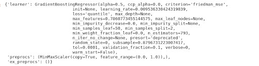
Another library that can be used for Bayesian optimization is Hyperopt. This package searches the hyper-parameter space based on the provided dataset. Before you can use it it needs to be installed from Github.
$ git clone git@github.com:hyperopt/hyperopt-sklearn.git
$ (cd hyperopt-sklearn && pip install -e .)
You can implement the same regression model by importing `gradient_boosting_regression` from `hpsklearn`. Next use the `HyperoptEstimator` and pass the following parameters:
- an Sklearn regressor,
- `max_evals` to dictate the maximum number of configurations,
- `trial_timeout` determines how many seconds the trial will run before it is killed, and the
- `algo` which is an hyperopt suggest algorithm e.g rand.suggest
from hyperopt import tpe
from hpsklearn import HyperoptEstimator,gradient_boosting_regression
regressor = HyperoptEstimator(regressor=gradient_boosting_regression('GradientBoostingRegressor'),
                          algo=tpe.suggest,
                          max_evals=100,
                          trial_timeout=300)
regressor.fit(X_train, y_train)
Once the fitting is done, the best hyper-parameters can be viewed.
regressor.best_model()
Since this is a Scikit-learn implementation, `refit` is set to True by default. This means that once the search is done the model is ready for use.
Another Bayesian package that we can look at is Optuna. After you have installed it, import it.
import optuna Next, define a function that will return the cross-validated score from the GradientBoostingRegressor. In the same function, define the parameters that you would like to search. As the parameters are defined, you also define the type:
- `suggest_int` refers to integer parameters,
- `suggest_categorical` categorical parameters, and
- `suggest_float` refers to float hyper-parameters
For the float and integer parameter types, the lower bound and the upper bound are specified.
from sklearn.model_selection import cross_val_score
def objective(trial):
  learning_rate = trial.suggest_float('learning_rate',0.01,0.3)
  max_depth = trial.suggest_int('max_depth',3,6)
  loss= trial.suggest_categorical('loss',['lad', 'ls','huber','quantile'])
  regressor = GradientBoostingRegressor(learning_rate=learning_rate,max_depth=max_depth)
  return cross_val_score(
        regressor, X_train, y_train, n_jobs=-1, cv=5,scoring='neg_root_mean_squared_error').mean()
After that a study object was created. As you do so, define the direction as `minimize` because you are focused on reducing the loss function. One of the parameters that can be passed as you create the study is the `sampler`. It dictates the background algorithm that will be used for value suggestion. If none is provided, the `optuna.samplers.TPESampler` is used. Other options for this are:
- `GridSampler` that uses grid search sampling,
- `RandomSampler ` that performs random sampling, and the
- `CmaEsSampler ` based on the CMA-ES algorithm.
The `TPESampler` uses the TPE (Tree-structured Parzen Estimator) algorithm.
After that you will call the `optimize` function as you pass in the function just created and the maximum number of trials.
study = optuna.create_study(direction='minimize')
study.optimize(objective, n_trials=20)
The best trial can be obtained from the `best_trial` attribute.
trial = study.best_trial
From that you can print the metrics as well as the best hyperparameters.
print('Root Mean Squared Error: {}'.format(trial.value))
print("Best Hyperparameters: {}".format(trial.params))
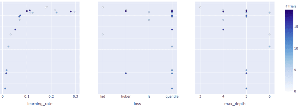
Furthermore, you can plot the optimization on a graph.
optuna.visualization.plot_optimization_history(study)

You can also plot the objective value for each trial.
Optuna also allows you to plot the hyper-parameter importances.
optuna.visualization.plot_param_importances(study)
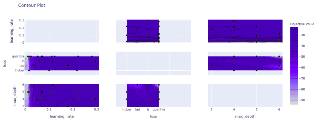
If you are interested in seeing the relationship between various parameters, you can do so using a contour plot.
optuna.visualization.plot_contour(study)
You might also want to save the experiment you were working on. You can do this by saving the study in pickle form.
import joblib
joblib.dump(study, 'study.pkl')
After this, you can version and track this in your experimentation platform.
Hyper-parameter Tuning in Deep Learning
You can also tune the parameters of your deep learning model. Let’s look at how this can be done using the classic MNIST example. For the tuning, we shall use the Keras Tuner package. Start by getting the normal imports out of the way.
from tensorflow import keras
from tensorflow.keras import layers
After this, you’ll need to import the search criteria that you would like to use. There are a couple of options:
- `RandomSearch` performs hyper-parameter tuning in a random manner,
- `Hyperband` uses adaptive resource allocation and early stopping in order to converge to a high performing model faster. The algorithm will train many models for a few epochs and settle on the top-performing models for the next round of training,
- `BayesianOptimization` that has already been covered,
- `Sklearn` used for tuning Scikit-learn Models.
In this case, let’s use the `RandomSearch` criteria.
from kerastuner.tuners import RandomSearch The next step is to define the deep learning model. Define the architecture of the model and pass in several options for the learning rate. This is the hyper-parameter that will be tuned in this example.
def build_model(hp):
    model = keras.Sequential()
    model.add(keras.layers.Flatten(input_shape=(28, 28)))
    model.add(layers.Dense(10, activation='softmax'))
    model.compile(
        optimizer=keras.optimizers.Adam(
            hp.Choice('learning_rate',
                      values=[1e-2, 1e-3, 1e-4])),
        loss='sparse_categorical_crossentropy',
        metrics=['accuracy'])
    return model
In the next step you’ll define the tuner and pass the following parameter to the tuner:
the model defined above,
the objective, in this case accuracy because we are solving a classification problem. Whether to maximize or minimize the objective function is automatically inferred for built in metrics,
`max_trials` that dictates the total that of trial that should be used for testing,
`executions_per_trial` is the maximum number of models that should be built and fit for every trial,
`directory` refers to the folder where the logs will be stored, and the
`project_name` is the name you would like to give your project.
tuner = RandomSearch(
    build_model,
    objective='val_accuracy',
    max_trials=5,
    executions_per_trial=3,
    directory='tunining',
    project_name='Hyper-parameter Tuning')
If you like, you can print a summary of your tuner.
tuner.search_space_summary() 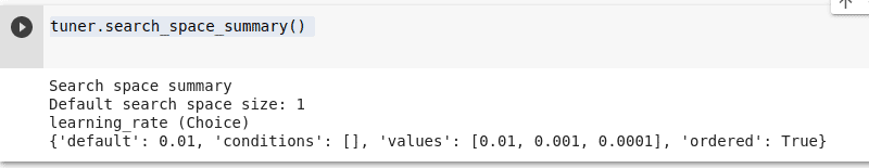
The next step is to run the search on the dataset. However, before you can do that, you have to obtain that dataset. You’ll use Keras to download the data and thereafter normalize it.
(X_train, y_train), (X_test, y_test) = keras.datasets.fashion_mnist.load_data()
X_train = X_train.astype('float32') / 255.0
X_test = X_test.astype('float32') / 255.0
Running the search is done using the `search` method of the tuner. As you do this you pass in the training set, the number of epochs and the validation set.
tuner.search(X_train, y_train,
             epochs=5,
validation_data=(X_test, y_test)) 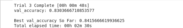
When the search is done, you can obtain the best models, in this case the top 3 are chosen.
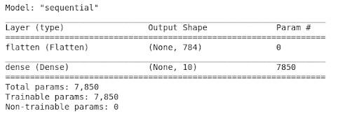
models = tuner.get_best_models(num_models=3) Let us look at the summary for the first model.
models[0].summary()
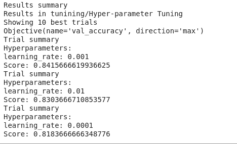
You can also take a look at the summary of the results obtained above. You can see that the image is showing the 10 best trials. As expected, the accuracy is being maximized.
tuner.results_summary()
How to track your training metrics with an AI platform
A common practice in the world of machine learning is to run various experiments and log the metrics. In this case one can also log the hyper-parameters used for each experiment. When using a platform like cnvrg.io the only thing you need to do is to pass the items to be logged via the `log_param` function. You can learn more about hyperparameter tuning and logging in the cnvrg.io documentation.
from cnvrg import Experiment
e = Experiment()
e.log_param("key", "value")
Once you have done this, the logged items will be available on your dashboard. This is important because you can keep track of all your parameters and stick with the ones that result in the best performance.
Conclusion
This article has covered various tools and techniques that can help you in adding hyper-parameter tuning to your machine learning pipeline. Specifically, some of the items covered are:
- What hyper-parameters are
- How hyper-parameters are different from model parameters
- What hyper-parameter tuning is
- Various strategies for adding hyper-parameter tuning to your ML workflow
- The different types of hyper-parameters
- How you can add hyper-parameter tuning to your deep learning models
Armed with this information, your model development and experimentation will be much easier.