Convolutional Neural Networks (CNN) have been used in state-of-the-art computer vision tasks such as face detection and self-driving cars. In this article, let’s take a look at the concepts required to understand CNNs in TensorFlow. Later you will also dive into some TensorFlow CNN examples.
What is CNN?
A Convolution Neural Network is a multi-layered artificial neural network that is capable of detecting complex features in data, for instance extracting features in image data.
How do CNNs work?
Although they can be used for other tasks, CNNs are mostly used in tasks involving image data. Each image contains pixel data that can be represented in a numerical form. This numerical representation is what is passed to a CNN. As much as normal artificial neural networks can be used in processing image data, CNNs have proven to perform better, resulting in higher accuracy. Let’s now take a look at how CNNs work.
Convolution
Usually, you will not feed the entire image to a CNN. You will feed the features that are most important in classifying the image. The features are obtained through a process known as convolution. The convolution operation results in what is known as a feature map. It is also referred to as the convolved feature or an activation map. The feature map is obtained by applying a feature detector to the input image. The feature detector is also referred to as a kernel or a filter. The filter is usually a 3 by 3 matrix. However, other types of matrices can be used. The feature map is obtained through an element-wise multiplication of the filter with the matrix representation of the input image. The objective here is to reduce the size of the image being passed to the CNN while maintaining the important features. The filter slides step by step through each of the elements in the input image. These steps are known as strides and can be defined when creating the CNN. When building the CNN you will be able to define the number of filters you want for your network.
Once you obtain the feature map, the Rectified Linear unit is applied in order to prevent the operation from being linear. This is because working with images is not linear.
Pooling
Pooling results in what is known as a pooled feature map. Pooling ensures that the neural network is able to detect features in an image irrespective of their location in an image. This is what is known as spatial invariance. There are several types of pooling, for example, max-pooling average pooling, and min pooling. For instance, in max-pooling a 2 by 2 matrix is slid over the feature map while picking the largest value in a given box.
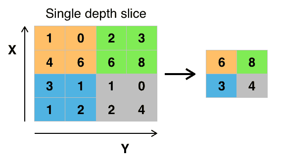
Pooling ensures that the main features of the image are maintained while reducing the size of the image further. This reduces the amount of information passed to the neural network and hence helps to reduce overfitting.
Flattening
The next step is to flatten the pooled feature map. This involves transforming the entire pooled feature map into a single column that can be passed to the fully connected layer.
Full connection
The flattened feature map is then passed to the input layer of the neural network. The result of that is passed to a fully connected layer. After that, the result of the entire process is emitted by the output layer. An activation function is usually applied depending on the type of classification problem. For binary classifications, the sigmoid activation function will be used whereas the softmax activation function is used for multiclass problems.
Architectures of CNNs
You don’t always have to design your convolutional neural networks from scratch. Other times one can try architectures developed by experts. These have proven to perform well on many image tasks. Some of these architectures are:
They can be accessed via Keras applications. These applications have also been pre-trained on the ImageNet dataset. The dataset contains over a million images. This makes these applications robust enough for use in the real world. When instantiating the model, you have the choice whether to include the pre-trained weights or not. When the weights are used, you can start using the model for classification right away. Other ways of using the pre-trained models are:
- extracting features and passing them to a new model
- fine-tuning a new model
Let’s take a look at how you can load the Xception architecture without weights. Since weights are not included, you can use your dataset to train the model.
					model = tf.keras.applications.Xception(
    include_top=True,
    input_tensor=None,
    input_shape=None,
    pooling=None,
    classes=1000,
    classifier_activation="softmax",
)
When you load the model with weights, you can start using it for prediction right away. The weights are stored in this location `~/.keras/models/`.
model = tf.keras.applications.Xception(
    include_top=True,
    weights="imagenet",
    input_tensor=None,
    input_shape=None,
    pooling=None,
    classes=1000,
    classifier_activation="softmax",
)
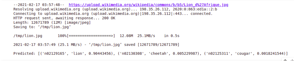
After that, you can process the image and run the predictions. The Keras applications provide a function for doing that. Each of the architectures dictates the size of the image that should be passed to it. You should always confirm that from its documentation. Next, convert the image into an array and expand its dimensions in order to include the batch size.
from tensorflow.keras.preprocessing import image
import numpy as np
!wget --no-check-certificate \
    https://upload.wikimedia.org/wikipedia/commons/b/b5/Lion_d%27Afrique.jpg \
    -O /tmp/lion.jpg
img_path = '/tmp/lion.jpg'
img = image.load_img(img_path, target_size=(299, 299))
x = image.img_to_array(img)
x = np.expand_dims(x, axis=0)
x = tf.keras.applications.xception.preprocess_input(x)

preds = model.predict(x)
# decode the results into a list of tuples (class, description, probability)
# (one such list for each sample in the batch)
print('Predicted:', tf.keras.applications.xception.decode_predictions(preds, top=3)[0])
The final step is to decode the predictions and print the results.
Convolutional Neural Networks (CNN) in TensorFlow
Now that you understand how convolutional neural networks work, you can start building them using TensorFlow. However, you will first have to install TensorFlow. If you are working on a Google Colab environment, TensorFlow will already be installed.
How to install TensorFlow
TensorFlow can be installed via pip. Run the following command to install it.
pip install tensorflow
Alternatively, you can run TensorFlow in a container.
 docker pull tensorflow/tensorflow:latest  # Download latest stable image
 docker run -it -p 8888:8888 tensorflow/tensorflow:latest-jupyter  # Start Jupyter server
How to confirm TensorFlow is installed
After installation is complete via pip, you might want to check TensorFlow’s version or confirm its installation. If you manage to import TensorFlow without any errors, then it was installed successfully.
import tensorflow
print(tensorflow.__version__)
What are Keras and tf.keras?
As of TensorFlow 2.0, Keras has become the official high-level API for TensorFlow. It is an open-source package that has been integrated into TensorFlow in order to quicken the process of building deep learning models. It is accessible via `tf.keras`. That is what you will be using in this article.
Develop multilayer CNN models
Let’s now take a look at how you can build a convolutional neural network with Keras and TensorFlow. The CIFAR-10 dataset will be used. The dataset contains 60000 32×32 color images in 10 classes, with 6000 images per class.
Develop multilayer CNN models
Loading the dataset can be done directly by using Keras utilities. Other datasets that ship with TensorFlow can be loaded in a similar manner.
(X_train, y_train), (X_test, y_test) = tf.keras.datasets.cifar10.load_data()
The dataset contains the following classes
'airplane', 'automobile', 'bird', 'cat', 'deer', 'dog', 'frog', 'horse', 'ship', 'truck'
You can use Matplotlib to visualize one of the images. Let’s visualize the image at index 785.
import matplotlib.pyplot as plt
image = X_train[785]
plt.imshow(image)
plt.show()
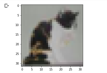
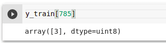
That looks like a cat. You can confirm that from the `y_train`. 3 is the label for a cat.
Data preprocessing
The weights of a neural network are initialized to very small numbers. Therefore, scaling the images to be within the same range is important. In this case, let’s scale the values to be numbers between 0 and 1.
X_train = X_train / 255
X_test = X_test / 255
Build the convolutional neural network
The next step is to define the convolutional neural network. Here is where the convolution, pooling, and flattening layers will be applied. The first layer is the `Conv2D`layer. It’s defined with the following parameters:
- 32 output filters
- a 3 by 3 feature detector
- `same` padding to result in even padding for the input
- input shape of `(32, 32, 3)` because the images are of size 32 by 32. 3 notifies the network that images are colored
- the `relu` activation function so as to achieve non-linearity
The next layer is a max-pooling layer defined with the following parameters:
- a `pool_size` of (2, 2) that defines the size of the pooling window
- 2 strides that define the number of steps taken by the pooling window
Remember that you can design your network as you like. You just have to monitor the metrics and tweak the design and settle on the one that results in the best performance. In this case, another convolution and pooling layer is created. That is followed by the flatten layer whose results are passed to the dense layer. The final layer has 10 units because the dataset has 10 classes. Since it’s a multiclass problem, the Softmax activation function is applied.
model = tf.keras.Sequential(
    [
    tf.keras.layers.Conv2D(32, (3,3), padding='same', activation="relu",input_shape=(32, 32, 3)),
    tf.keras.layers.MaxPooling2D((2, 2), strides=2),

    tf.keras.layers.Conv2D(64, (3,3), padding='same', activation="relu"),
    tf.keras.layers.MaxPooling2D((2, 2), strides=2),

    tf.keras.layers.Flatten(),
    tf.keras.layers.Dense(100, activation="relu"),
    tf.keras.layers.Dense(10, activation="softmax")
]
)
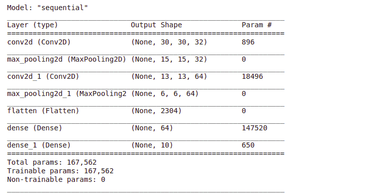
How to visualize a deep learning model
The quickest way to visualize your model is to use the model summary function.
model.summary()
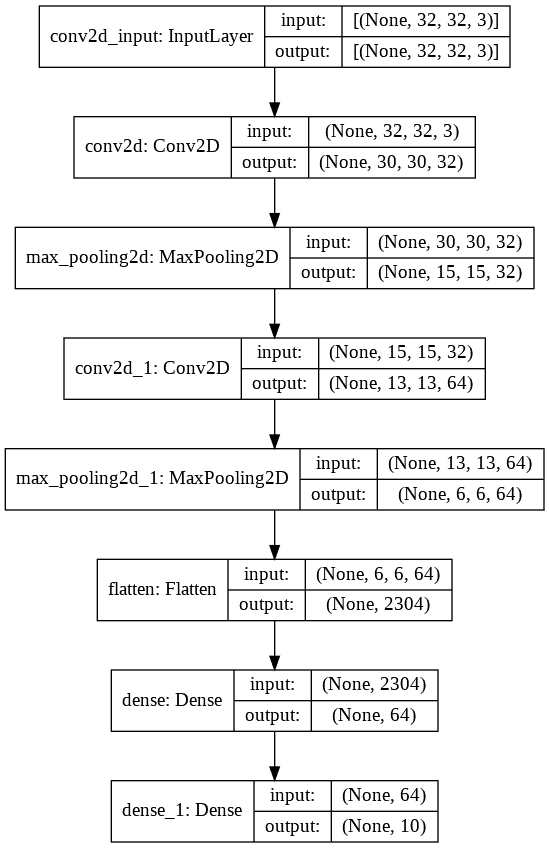
You can also use the Keras `plot_model` utility to plot the model.
tf.keras.utils.plot_model(
    model,
    to_file="model.png",
    show_shapes=True,
    show_layer_names=True,
    rankdir="TB",
    expand_nested=True,
    dpi=96,
)
How to reduce overfitting with Dropout
One of the common ways to improve the performance of deep learning models is to introduce dropout regularization. In this process, a specified percentage of connections are dropped during the training process. This forces the network to learn patterns from the data instead of memorizing the data. This is what reduces overfitting. In Keras, this can be achieved by introducing a Dropout layer in the network. Here is how the network would look like after applying the DropOut layer.
model = tf.keras.Sequential(
    [
    tf.keras.layers.Conv2D(32, (3,3), padding='same', activation="relu",input_shape=(32, 32, 3)),
    tf.keras.layers.MaxPooling2D((2, 2), strides=2),

    tf.keras.layers.Conv2D(64, (3,3), padding='same', activation="relu"),
    tf.keras.layers.MaxPooling2D((2, 2), strides=2),

    tf.keras.layers.Flatten(),
    tf.keras.layers.Dense(100, activation="relu"),
    tf.keras.layers.Dropout(0.2),
    tf.keras.layers.Dense(10, activation="softmax")
]
)
Compiling the model
The next step is to compile the model. The Sparse Categorical Cross-Entropy loss is used because the labels are not one-hot encoded. In the event that you want to encode the labels, then you will have to use the Categorical Cross-Entropy loss function.
model.compile(optimizer='adam',
              loss=tf.keras.losses.SparseCategoricalCrossentropy(from_logits=True),
              metrics=['accuracy'])
How to halt training at the right time with Early Stopping
Left to train for more epochs than needed, your model will most likely overfit on the training set. One of the ways to avoid that is to stop the training process when the model stops improving. This is done by monitoring the loss or the accuracy. In order to achieve that, the Keras EarlyStopping callback is used. By default, the callback monitors the validation loss. Patience is the number of epochs to wait before stopping the training process if there is no improvement in the model loss. This callback will be used at the training stage. The callbacks should be passed as a list, even if it’s just one callback.
from tensorflow.keras.callbacks import EarlyStopping
callbacks = [
             EarlyStopping(patience=2)
]
How to save the best model automatically
You might also be interested in automatically saving the best model or model weights during training. That can be applied using a Keras ModelCheckpoint callback. The callback will save the best model after each epoch. You can instruct it to save the entire model or just the model weights. By default, it will save the models where the validation loss is minimum.
checkpoint_filepath = '/tmp/checkpoint'
model_checkpoint_callback = tf.keras.callbacks.ModelCheckpoint(
    filepath=checkpoint_filepath,
    save_weights_only=False,
    monitor='loss',
    mode='min',
    save_best_only=True)
Your callbacks will now look like this.
callbacks = [
             EarlyStopping(patience=2),
             model_checkpoint_callback,
]
After training, you can load the model again using the Keras `load_model` utility.
another_saved_model = tf.keras.models.load_model(checkpoint_filepath)
Training the model
Let’s now fit the data to the training set. The validation set is passed as well because the callback monitors the validation set. In this case, you can define many epochs but the training process will be stopped by the callback when the loss doesn’t improve after 2 epochs as declared in the EarlyStopping callback.
history = model.fit(X_train,y_train, epochs=600,validation_data=(X_test,y_test),callbacks=callbacks)
How to plot model learning curves
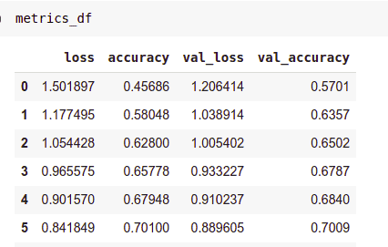
Learning curves are important because they can inform you whether the model is learning or overfitting. If the validation loss increases significantly or the validation accuracy reduces sharply then your model is most likely overfitting. Since the model was saved into a history variable, you can use that to access the losses and accuracy and plot them. You can also store them in a Pandas DataFrame.
					import pandas as pd
metrics_df = pd.DataFrame(history.history)
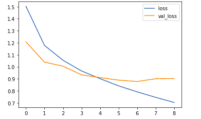
Let’s now look at how you would plot the training and validation loss.
metrics_df[["loss","val_loss"]].plot();
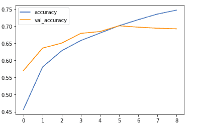
The same can be done for the training and validation accuracy.
metrics_df[["accuracy","val_accuracy"]].plot();
How to save and load your model
You might be interested in saving the model for later use. Saving the model is important so that you don’t have to train the model again. This is especially critical for image models that take a long period to train. The H5 format is a common format for saving Keras models.
model.save(“model.h5”)
The Keras `load_model` is used for loading the model again.
load_saved_model = tf.keras.models.load_model("model.h5")
load_saved_model.summary()
How to accelerate training with Batch Normalization
The network you trained here was relatively small. However, in other cases, you might have to train a very deep neural network. Training such a network can be very slow. The training process can be hastened using Batch Normalization. It transforms the data ensuring that the mean output is closer to zero and the output standard deviation is close to 1. The mean and variance are computed using the current batch of inputs. Since Batch Normalization offers some form of regularization it is usually not used with DropOut. Here’s how the model would look like after adding the batch normalization layer.
					model = tf.keras.Sequential(
    [
    tf.keras.layers.Conv2D(32, (3,3), padding='same', activation="relu",input_shape=(32, 32, 3)),
    tf.keras.layers.MaxPooling2D((2, 2), strides=2),

    tf.keras.layers.Conv2D(64, (3,3), padding='same', activation="relu"),
    tf.keras.layers.MaxPooling2D((2, 2), strides=2),

    tf.keras.layers.Flatten(),
    tf.keras.layers.Dense(100, activation="relu"),
    tf.keras.layers.BatchNormalization(),
    tf.keras.layers.Dense(10, activation="softmax")
]
The working of the batch normalization layer is different during training and during prediction and evaluation. During training `trainable=True` while during prediction and evaluation it’s false. When training normalization is done using the mean and standard deviation of the current batch of inputs. At inference i.e prediction and evaluation, normalization is done using a moving average of the mean and the standard deviation of the batches seen during training. When using a pre-trained model that contains this layer, training for the batch normalization layer has to be set to false. Otherwise the mean and standard deviation will be disrupted and all the prior learning lost.
Running CNNs with TensorFlow in the real world
Loading datasets from TensorFlow is quite straightforward. However, consider a situation where you have to load data from the real world. The process for doing so is a little different. In this section, let’s look at how you can use this dataset from Kaggle to build a convolutional neural network. The goal here will be to build a model that can classify images of cats and dogs. Once you have built this model, you can tweak it and repurpose it for other classification problems.
Loading the images
Let’s start by downloading the images into a temporary folder on the virtual machine provided by Google Colab. Using Colab, in this case, is advantageous because you can use GPU compute to speed the model training.
!wget --no-check-certificate \ https://namespace.co.ke/ml/dataset.zip \ -O /tmp/catsdogs.zip
The next step will be to unzip this dataset.
import os
import zipfile
with zipfile.ZipFile('/tmp/catsdogs.zip', 'r') as zip_ref:
    zip_ref.extractall('/tmp/cats_dogs')
After that set the paths to the training and testing set.
base_dir = '/tmp/cats_dogs/dataset'
train_dir = os.path.join(base_dir, 'training_set')
test_dir = os.path.join(base_dir, 'test_set')
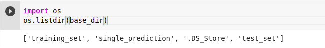
You can list the folders in order to see their arrangement.
import os
os.listdir(base_dir)
Generates a tf.data.Dataset
The next step is to create a TensorFlow dataset from the images. That can be done using the `image_dataset_from_directory`. Since it will infer the classes from the folder, your data should be structured as shown below.
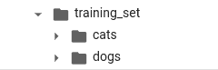
When using the function to generate the dataset, you will need to define the following parameters:
- the path to the data
- an optional seed for shuffling and transformations
- the `image_size` is the size the images will be resized to after being loaded from the disk
- since this is a binary classification problem the `label_mode` is binary
- `batch_size=32` means that the images will be loaded in batches of 32
In the absence of a validation set, you can also define a `validation_split`. If it is set, the `subset` also needs to be passed. That is to indicate whether the split is a validation or training split. In this case, let’s use the testing set for validation.
					training_set = tf.keras.preprocessing.image_dataset_from_directory(
  train_dir,
  seed=101,
  image_size=(200, 200),
  batch_size=32)
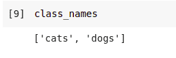
By default, the classes will be represented using integers. You can see the representation by using `class_names` of the generated training set.
class_names = training_set.class_names
In this case, cats will be represented by 0 and dogs by 1.This is based on the directory structure of the dataset. Since `class_names` isn’t specified, the alphanumerical order will be used.
Generate the validation split as well. The arguments are similar to the training set;
- the directory containing the images
- an optional seed
- how to resize the images
- the size of the batches
					validation_set = tf.keras.preprocessing.image_dataset_from_directory(
  test_dir,
  seed=101,
  image_size=(200, 200),
  batch_size=32)
Data augmentation
Data augmentation is usually applied in order to prevent overfitting. Augmenting the images increases the dataset as well as exposes the model to various aspects of the data. Augmentation can be achieved by applying random transformations such as flipping and rotating the images. Fortunately, Keras provides layers that can do just that.
data_augmentation = keras.Sequential(
  [
    tf.keras.layers.experimental.preprocessing.RandomFlip("horizontal",
                                                 input_shape=(200,                                                           200,
                                                               3)),
    tf.keras.layers.experimental.preprocessing.RandomRotation(0.2),
    tf.keras.layers.experimental.preprocessing.RandomZoom(0.2),
  ]
)
Model definition
Let’s now create the convolutional neural network that will be used to classify the images. It will be similar to the previous one with a few cosmetic changes.
import tensorflow as tf
from tensorflow import keras
from tensorflow.keras import Sequential
from tensorflow.keras.layers import Dense,Conv2D,MaxPooling2D,Flatten,Dropout
from tensorflow.keras.preprocessing.image import ImageDataGenerator
model = Sequential([
    data_augmentation,
    tf.keras.layers.experimental.preprocessing.Rescaling(1./255),
    Conv2D(filters=32,kernel_size=(3,3), activation='relu'),
    MaxPooling2D(pool_size=(2,2)),

    Conv2D(filters=32,kernel_size=(3,3), activation='relu'),
    MaxPooling2D(pool_size=(2,2)),
    Dropout(0.25),

    Conv2D(filters=64,kernel_size=(3,3), activation='relu'),
    MaxPooling2D(pool_size=(2,2)),
    Dropout(0.25),

    Flatten(),
    Dense(128, activation='relu'),
    Dropout(0.25),
    Dense(1, activation='sigmoid')
])
The notable changes are:
- the application of the augmentation layer
- using the `Scaling` layer to scale the images in the model definition
Compiling the model
Let’s now compile the model. Since it’s a binary problem, the `BinaryCrossentropy` and the `BinaryAccuracy` can be used.
model.compile(optimizer='adam',
              loss=keras.losses.BinaryCrossentropy(from_logits=True),
              metrics=[keras.metrics.BinaryAccuracy()])
Training the model
The next step is to train the model. In this case, `y` is not passed in. That’s taken care of by the function used to generate the training set. Passing the validation data is critical so that the loss and accuracy can be accessed later and plotted. Let’s also reuse the callbacks that were defined in the last section.
history = model.fit(training_set,validation_data=validation_set, epochs=600,callbacks=callbacks)
Monitoring the model’s performance
Using the history object, the training losses and accuracies can be obtained.
import pandas as pd

metrics_df = pd.DataFrame(history.history)
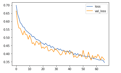
You can plot them in order to see the learning curves. Let’s start by comparing the training and validation loss.
metrics_df[["loss","val_loss"]].plot();
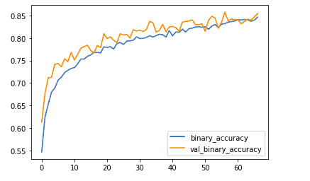
Next, on to the training and validation accuracy.
metrics_df[["binary_accuracy","val_binary_accuracy"]].plot();
Model evaluation
You can also check the performance of the model on the validation set.
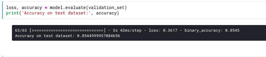
loss, accuracy = model.evaluate(validation_set)
print('Accuracy on test dataset:', accuracy)
Let’s now try the model on new images. The `image` module from Keras will be used to load the image.
import numpy as np
from keras.preprocessing import image
Download some images from the internet and store them in a temporary folder. The images used here are provided via the permissive creative commons license.
!wget --no-check-certificate \
    https://upload.wikimedia.org/wikipedia/commons/c/c7/Tabby_cat_with_blue_eyes-3336579.jpg \
    -O /tmp/cat.jpg
Next, load the image while specifying the size used in training.
test_image = image.load_img('/tmp/cat.jpg', target_size=(200, 200))
After this, convert it into an array since the model expects array inputs.
test_image = image.img_to_array(test_image)
The next step is to expand the dimensions of the image in order to include the batch size. Let’s take a look at the shape of the image at the moment.
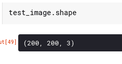
That needs to be amended to include a batch size of 1, because only one image is being used here. Expanding the dimensions is done using the `expand_dims` function from NumPy.
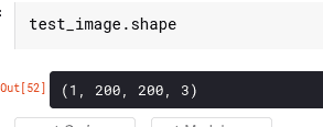
test_image = np.expand_dims(test_image, axis=0)
If you check the shape again, you will see that it’s in the form required by the model.
Making predictions
You can now use this image to run a prediction.
prediction = model.predict(test_image)
When you print this you will see something similar to this.
prediction[0][0]
0.014393696
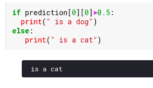
The question is, how do you interpret this? Remember that the network output layer has just one unit and uses the sigmoid activation function. The output of this network is therefore a number between 0 and 1. That number represents the probability that the image belongs to class 1. Class 1 in this case is dogs. You can therefore set a threshold of say 50% to separate the two classes.
if prediction[0][0]>0.5:
  print(" is a dog")
else:
   print(" is a cat")
Since the obtained probability is less than 0.5 then that image is definitely that of a cat.
You can repeat the same process with a dogs image. First, start by downloading the image.
!wget --no-check-certificate \
    https://upload.wikimedia.org/wikipedia/commons/1/18/Dog_Breeds.jpg \
    -O /tmp/dog.jpg
After that, load it while converting it to the required size.
test_image2 = image.load_img('/tmp/dog.jpg', target_size=(200, 200))
Next, expand the dimensions and run the prediction.
test_image2 = np.expand_dims(test_image2, axis=0)
prediction = model.predict(test_image2)
Use the same threshold to determine if it is the image of a cat or a dog.
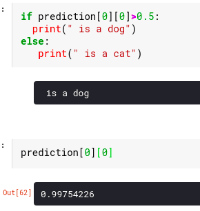
if prediction[0][0]>0.5:
  print(" is a dog")
else:
   print(" is a cat")
With an accuracy of 99%, the image is classified as a dog.
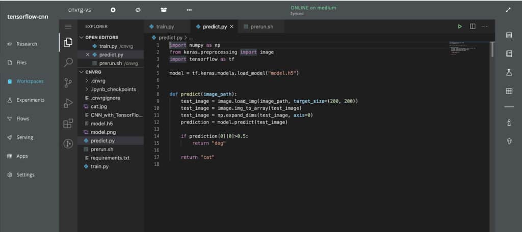
How to easily run CNN with Tensorflow in cnvrg.io
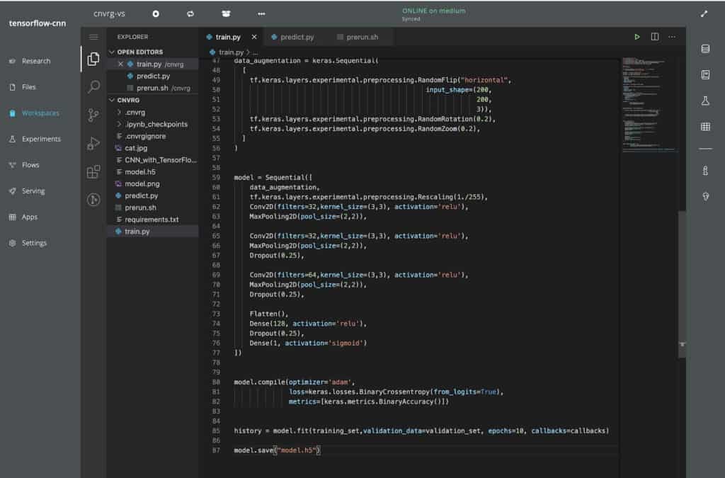
Now, with cnvrg.io you can run this pipeline without configuring the different platforms which makes it much faster and easier to run. Using cnvrg.io, you can easily track training progress and serve the model as a REST endpoint. First, you can spin up a VS Code workspace inside cnvrg.io to build our training script from the notebook code. You can use the exact code and ensure that the model is saved at the end of the training.
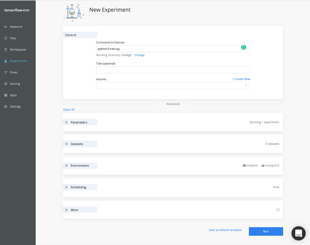
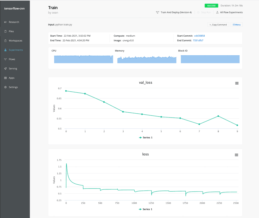
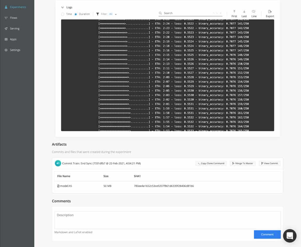
Run your code as an experiment
Next, you can launch this training script as an experiment. cnvrg.io will provision resources to execute the script and monitor the performance automatically. Resource and training metrics are automatically visualized along with the logs, and all files that were written to disk during the experiment are saved as artifacts in cnvrg.io’s object store.
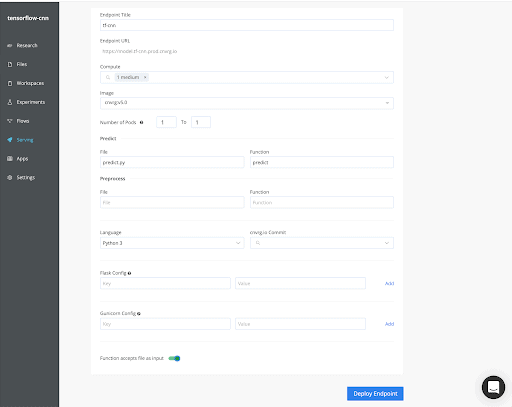
Make predictions in a few clicks
Now that you have your model, you’ll need to create a “predict” function. cnvrg.io makes it easy, by automatically wrapping this function into a production-grade Flask application equipped with load balancing, autoscaling, monitoring. This file loads the model into memory and uses it in the predict function, which will format the incoming data and return a prediction.
Deploy your predictions to an endpoint
Next, you’ll want to create an endpoint that routes to that function. You could also specify compute resources and autoscaling configurations here too.
Track and monitor your endpoints
cnvrg.io automatically displays metrics such as the number of requests and latency for the endpoint. It also comes with Grafana and Kibana integrated for increased visibility into model
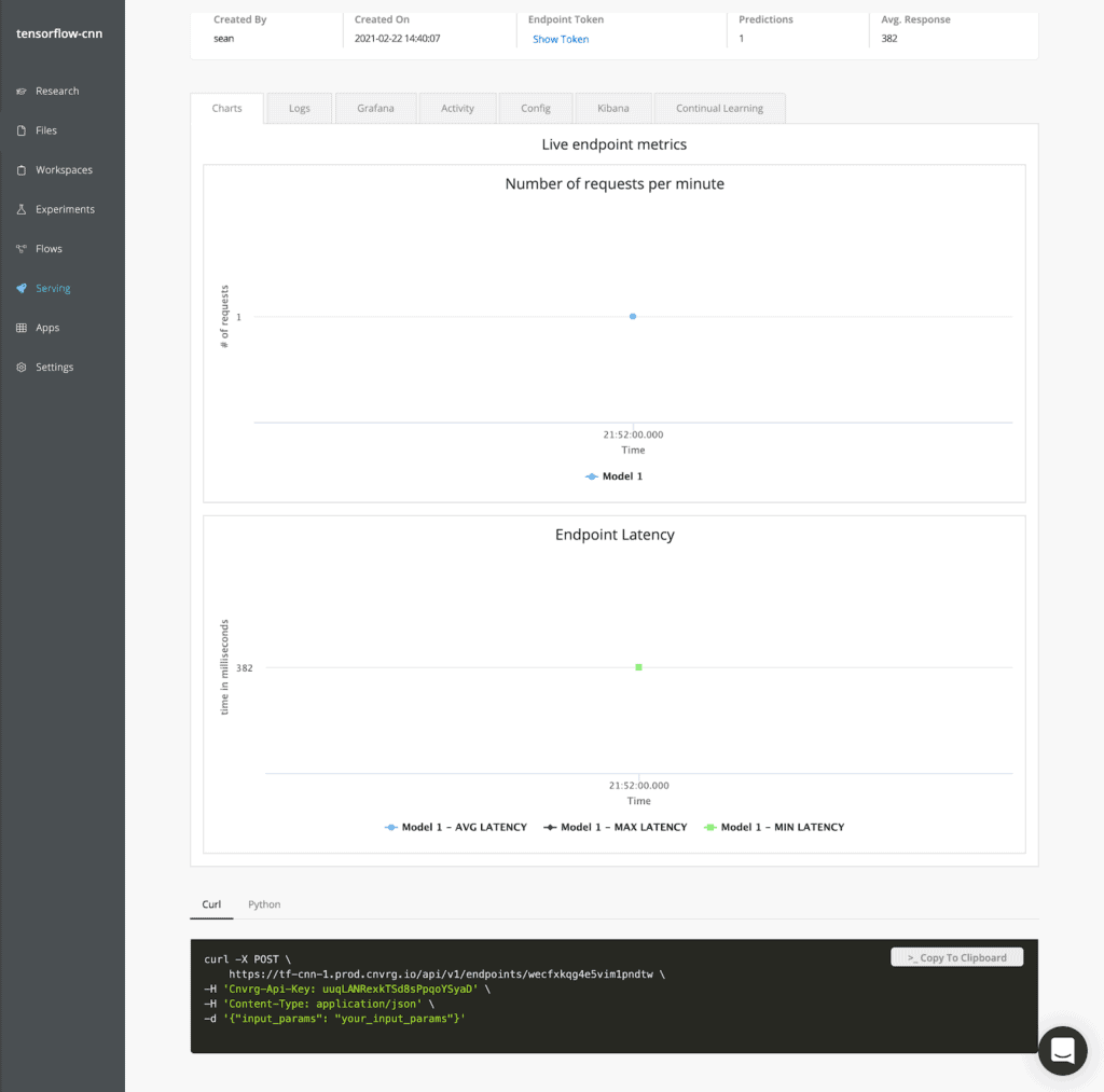
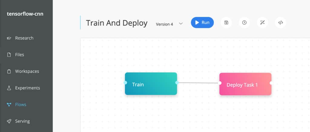
Finally, if you want to trigger retraining and deploying the model as part of a CI/CD pipeline, cnvrg.io provides Flows. The pipeline could programatically trigger the flow via cnvrg.io’s CLI or SDK.
You can test it out in cnvrg.io now by installing cnvrg.io CORE our free community MLOps platform on your Kuberentes here.
Final remarks
In this article, you have learned CNNs from their intuition to their applications in the real world. You have also seen that you can use existing architectures to hasten your model development process. Specifically, you have covered:
- what convolutional neural networks are
- how convolutional neural networks work
- using pre-trained convolutional neural networks to run image classification
- building convolutional neural networks from scratch using Keras and TensorFlow
- how to plot the learning curves of your neural network
- preventing overfitting using DropOut regularization and batch normalization
- saving your best model using the model checkpoint callback
- how to stop the training process of your CNN when it stops improving
- how you can save and load the model again
…just to mention a few.
And that’s not the end of it, you can explore all the examples used in this article on this Google Colab Notebook. Feel free to play with the parameters of the models to see how they affect the performance of the model.