
Bin packing involves packing a set of items of different sizes in containers of various sizes. The size of the container shouldn’t be bigger than the size of the objects. The goal is to pack as many items as possible in the least number of containers possible. Generally speaking, this is referred to as an optimization problem.
This article will focus on the bin packing problem. This concept is important to understand due to its applicability in resource allocation in ML orchestration. In computing this is applicable in resource allocations e.g GPU as well as scheduling of processes. Let’s start by discussing that.
GPU utilization with bin packing
Serving Deep Neural Networks (DNNs) efficiently from a cluster of GPUs is a problem that can be addressed via bin packing. This is important in order to ensure high utilization as well as low-cost GPU usage. Achieving this requires cluster-scale resource management; for instance, scheduling of GPUs.The ability to distribute a large workload onto a cluster at a high accelerator utilization and acceptable latency is therefore critical. The application of packing-based scheduling algorithms can be used to address this issue. The schedule can specify three items:
- the needed GPUs
- the distribution of neural nets across them
- their execution order that guarantees high throughput and low latency
Loading models into memory consumes a lot of time. When served at high velocity, the models can first be pre-loaded into a GPU memory. This can then be re-used in future executions. Placing these models requires efficient packing. It is important to note that in most deep learning systems data is passed in batches. This improves GPU utilization but poses problems in the allocation of resources in a cluster. The problems arise from the fact that the process cost of input depends on the size of the batch where the input is being processed. The algorithm that is packing the models in the GPUs has to take this into consideration. Generally, this is known as batching-aware resource allocation.
Another issue that needs to be taken into consideration is where there are few model requests. These requests don’t necessarily need a GPU. In order to optimize resource utilization, these requests can be packed into a single GPU. This is an optimization problem that can be denoted as an integer programming problem. Some of the constraints on this problem include:
- the required latency
- only GPUs that are in use can be assigned
- only one GPU can be assigned to each session
One of the libraries that can be used for this problem is the CPLEX package. Since solving this integer problem is computationally expensive, greedy scheduling algorithms can be considered.
Bin packing can also be applied in training convolutional neural networks with GPUs in order to ensure efficient training. This is achieved by allocating CNN layers to computational units. The objective, in this case, is to minimize the overall training time. The First-Forward Decreasing (FFD) algorithm can be used to map layers to the bins. Since it is a greedy algorithm it will place items in bins in decreasing order of their size.
Before we go any further, it is worthy to briefly mention other optimization problems.
Optimization problems
In optimization, the aim is to obtain the best possible solution out of a huge set of possible options. For example, in the computing world, you may be interested in assigning resources to a certain project. In this case, your goal is to use the optimal number of resources sufficient for the project as well as the most cost-effective. Essentially, you don’t want to purchase resources that will not be used. You are therefore trying to ensure that there is no wastage of resources.
Types of optimization problems
The first step in solving any optimization problem is to identify its type. The next step is to find the best algorithm that will obtain the optimal solution. Let’s now mention a couple of optimization problems.
Routing
This problem involves finding the most optimal route in the delivery of packages to customers. You, therefore, have to assign packages and routes to trucks in a manner that minimizes the total cost of delivery.
Assignment
In this case, workers have to be assigned to tasks that involve a fixed cost. The goal here is to make the assignment that leads to the least cost.
Packing
In packing problems, containers with fixed sizes are provided. Given a set of items, the goal is to find the best way to pack the objects. In a packing problem, the goal is to maximize or minimize something. For instance, one could be interested in maximizing the total value of the packed items or minimizing the cost of shipping the items. There are two main variants of packing; knapsack problems and bin packing. The simple knapsack problem involves just one container. In this case, the goal is to pack the items that result in the total maximum value. A variant of the knapsack problem known as the multiple knapsack problem is concerned with maximizing the total value of the packed items in all knapsacks.
The bin-packing problem
n this case, multiple containers of the same capacity are provided. They are usually referred to as bins. The aim is to compute the least number of bins that can hold all the items. The number of bins is not fixed. This is different from the multiple knapsack problem where the number of containers is fixed. For instance, let’s illustrate this using that shipping problem. In a bin packing problem, you have more than enough trucks to ferry all the items but you want to make sure that you use the least number of trucks to hold all the items. However, in the multiple knapsack problem, you have a fixed number of trucks and your goal is to load a subset of the packages that will result in the maximum weight.
As you have seen so far, optimization involves two main things; the objective and the constraints. The objective is the quantity that you are optimizing, for instance, the number of trucks in the shipping example. The constraints are the set restrictions, for example, the total number of trucks available. In order to solve any optimization problem you first need to identify the objective and the constraints. The optimal solution is the one that meets the objective whereas the feasible solution is the one that satisfies the given constraints even if it’s not optimal. The goal is always to aim for the optimal solution.
Bin packing algorithms
The bin packing problem can be solved by algorithms. These algorithms can either be online or offline heuristic.
Online heuristics
In online heuristics items arrive in order. As they come a decision of whether to pack an item must be made. The algorithm does not have any information about the next item or if there will be a next item.
Next-Fit
In this algorithm, there is only one bin that is partially filled at any time. The algorithm works by considering items in an ordered list. An item is placed in the same bin as the previous item if it fits there. If it doesn’t fit in the bin, that bin is closed. A new bin is opened and the item is placed inside the new bin.
For instance, if you’ve just placed an item in bin 5, then you will never put anything in bin 1-4. If there is a next item it will go to bin 5 if it fits there. If it doesn’t fit into the 5th bin it will go into the 6th
Next-k-Fit
This algorithm works like the above one but keeps the last k bins open and selects the bin in which the item fits.
First-Fit
In this algorithm, items are processed in an arbitrary order. The algorithm tries to place an item in the first bin that can hold the item. In the event that no bin is found, a new bin is opened and the item is placed in the new bin.
So an item will be placed in bin 1 if it fits there, if it doesn’t, it is placed in bin 2. If the item doesn’t fit in a bin that already contains an item, then a new bin is opened.
Best-Fit
This algorithm is similar to the previous one. The difference is that it doesn’t place the next item in the first bin where it fits. If the item fits, it is placed in the bin with the maximum load.
Worst-Fit
This algorithm is similar to the previous one. The difference is that instead of placing the item in the bin that has the maximum load, it is placed in the bin with the minimum load. A new bin is opened if the item doesn’t fit in that bin. If there are two bins with the same minimum load then the one that was opened earliest is used.
Almost Worst-Fit
This algorithm works by examining the order of the list and attempts to place the next item in the second most empty open bin. If the item doesn’t fit the algorithm, then it tries to place the item in the most empty bin. If it doesn’t fit there, the algorithm will open a new bin.
Offline heuristics
Offline heuristic algorithms have complete information about the items before execution. As a result, they have the ability to modify the order of the list of items.
First Fit Decreasing
This one is similar to First-Fit. The difference is that items are sorted in non-increasing order of their sizes before they are placed.
Optimization solvers
There are also Python packages that can be used to solve the bin packing problem. The process of solving the problem entails:
- defining a solver
- declaring the constraints
- defining the objective function
- showing the result
Let’s take a look at solving the problem in Python.
OR-Tools
OR-Tools is an open-source library for combinatorial optimization. It can be used to solve the scheduling problem, vehicle routing as well as the bin packing problem.
Let’s start by importing the library and declaring the solver. The solver is a mixed-integer programming solver.
from ortools.linear_solver import pywraplp
solver = pywraplp.Solver.CreateSolver(“SCIP_MIXED_INTEGER_PROGRAMMING”)
`pywraplp` is a Python wrapper for the C++ linear solver wrapper. In this case, the SCIP backend is used.
Next, define the data that you would like to use:
- `weights` is a list containing the weights of the items
- `bin_capacity` is the capacity of the bins
Since the goal is to minimize the number of bins, no value is assigned to the items.
def define_data():
    data = {}
    data['weights'] = [45, 50, 12, 70, 120, 78, 89, 20, 30, 17, 59]
    data['items'] = [0, 1, 2, 3, 4, 5, 6, 7, 8, 9, 10]
    data['bins'] = data['items']
    data['bin_capacity'] = 150
    return data
data = define_data()
The next step is to declare the program’s variables:
- `x[i, j]` is equal to 1 if item i is packed in bin j, otherwise, it’s 0
- `y[j]`is defined as 1 if bin j is used, otherwise, it’s 0
The sum of `y[j]` is the total number of bins used.
x = {}
for i in data['items']:
    for j in data['bins']:
        x[(i, j)] = solver.IntVar(0, 1, 'x_%i_%i' % (i, j))

y = {}
for j in data['bins']:
    y[j] = solver.IntVar(0, 1, 'y[%i]' % j)
The next step is to define the program constraints. The first constraint is that each item should be in exactly one bin. This is set by ensuring that the sum of `x[i][j]` overall bins j is equal to 1.
for i in data['items']:
    solver.Add(sum(x[i, j] for j in data['bins']) == 1)
The next constraint is that the total weight packed in each bin should not exceed the capacity of the bin.
for j in data['bins']:
    solver.Add( sum(x[(i, j)] * data['weights'][i] for i in data['items']) <= y[j] *  data['bin_capacity'])
The next step is to define the objective function. The objective, in this case, is to reduce the number of bins. This is enforced by minimizing the sum of the y[j] which is the number of bins used.
solver.Minimize(solver.Sum([y[j] for j in data['bins']])) Finally, call the solver and display the solution.
status = solver.Solve()
if status == pywraplp.Solver.OPTIMAL:
num_bins = 0.
for j in data['bins']:
if y[j].solution_value() == 1:
bin_items = []
bin_weight = 0
for i in data['items']:
if x[i, j].solution_value() > 0:
bin_items.append(i)
bin_weight += data['weights'][i]
if bin_weight > 0:
num_bins += 1
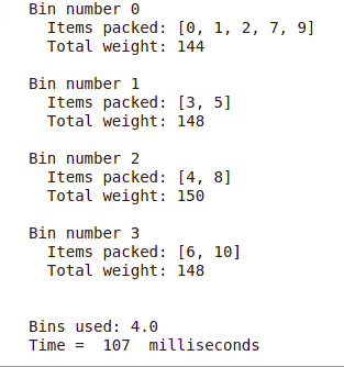
print('Bin number', j)
print(' Items packed:', bin_items)
print(' Total weight:', bin_weight)
print()
print()
print('Bins used:', num_bins)
print('Time = ', solver.WallTime(), ' milliseconds')
else:
print('Problem has no optimal solution.') In the solution, you will see the least number of bins needed to pack all the items. It also shows the items packed in each bin that was used as well as the total bin weight.
Binpacking
Another package that you can look at is binpacking. It uses greedy algorithms to solve bin packing problems in two main ways:
- sorting items in a constant number of bins
- sorting items into a low number of bins of constant size
Let’s start by looking at the first scenario. First, import the package and declare the resources. Contributions are defined in a dictionary with the key being the name of the resource and the values being its contribution value.
import binpacking

b = { 'a': 12, 'b': 21, 'c':11, 'd':31, 'e': 22,'f':17 }
The items can be sorted into constant bins by using the `to_constant_bin_number` function. The function accepts the dictionary of the resources and the number of bins expected.
bins = binpacking.to_constant_bin_number(b,5)
bins 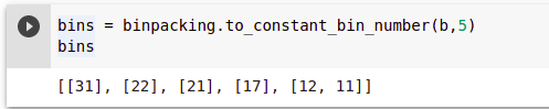
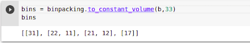
Sorting the items into a low number of bins of constant size is achieved by using the `to_constant_volume`. The function accepts a list containing weights and the maximum expected volume.
b = list(b.values())
bins = binpacking.to_constant_volume(b,33)
bins
Final Thoughts
In this article, you have seen that there are various variants of the bin packing problem. You have also learned about the algorithms and optimization solvers that can be used to solve the bin packing problem. Specifically, you have covered:
- various types of optimization problems
- what the bin packing problem is
- online and offline algorithms for solving the bin packing problem
- solving the problem using OR-Tools and the bin packing packages
- GPU utilization of bin packing
just to mention a few. The examples used here can be found in this Google Colab Notebook.