In this article, we’ll take a deep dive into the world of semantic segmentation. Some of the items that will be covered include:
- What is semantic segmentation
- The difference between image segmentation and instance segmentation
- Popular image segmentation architectures
- Image segmentation loss functions
- Data augmentation for image segmentation
- Semantic segmentation implementation in Python
What is semantic segmentation?
The process of linking each pixel in an image to a class label is referred to as semantic segmentation. The label could be, for example, cat, flower, lion etc. Semantic segmentation can be thought of as image classification at pixel level. Therefore, in semantic segmentation, every pixel of the image has to be associated with a certain class label.
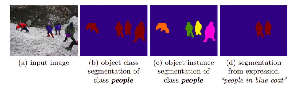
Semantic segmentation vs. Instance segmentation
Let’s take an example where we have an image with six people. Object detection would identify the six people and give them a single label of person by creating bounding boxes around them. Semantic segmentation goes further and creates a mask over each person that was identified and gives all of them a single label of person. In instance segmentation, every instance a person gets its own label.

Semantic Segmentation Use Cases
Semantic segmentation is used in areas where thorough understanding of the image is required. Some of these areas include:
- diagnosing medical conditions by segmenting cells and tissues
- navigation in self-driving cars
- separating foregrounds and backgrounds in photo and video editing
- developing robots that can move and interact with objects in their environment
In these cases, precise pixel-level understanding of the environment is critical.
Semantic Segmentation Approaches
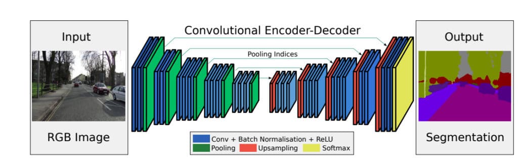
One of the approaches used in image segmentation is the encoder -decoder method. The encoder is made up of a set of layers that extract features from an image using filters. In many cases, the encoder is pre-trained in a task such as image classification where it learns the correlations from multiple images. This knowledge can then be transferred during the process of image segmentation. The final output, which is a segmentation mask, is generated by the decoder. The decoder is made of layers whose responsibility is to generate the final output. The decoder also ensures that the generated mask bears resemblance to the pixel resolution of the input image.
In this article you will see that there are several approaches used in the decoder, namely:
- Region-Based Semantic Segmentation
- Fully Convolutional Network-Based Semantic Segmentation
- Weakly Supervised Semantic Segmentation
6 Useful Image Segmentation Datasets
Working with image segmentation has been made easier by the availability of image segmentation datasets. Furthermore, some of them are already packaged in your favorite deep learning framework.
Coco
Coco is a large scale image segmentation and image captioning dataset. It is made up of 330K images and over 200K are labeled. It contains 80 object categories and 250K people with key points. When working with TensorFlow, you can easily import Coco into your work environment. First you will need to ensure that `tensorflow_datasets` is installed. You can do that via `pip`. After that the dataset can be loaded as shown below.
import tensorflow_datasets as tfds
(X_train, X_test), ds_info = tfds.load(
    'coco',
    split=['train', 'test'],
    shuffle_files=True,
    as_supervised=True,
    with_info=True,
)
PASCAL Visual Object Classes (PASCAL VOC)
This is a dataset from the PASCAL Visual Object Classes Challenge. It contains 20 different classes and 24640 annotated objects. In total, the dataset contains 9963 images. In TensorFlow, it can be loaded as shown below:
import tensorflow_datasets as tfds
(X_train, X_test), ds_info = tfds.load(
    ‘voc’,
    split=['train', 'test'],
    shuffle_files=True,
    as_supervised=True,
    with_info=True,
)
Waymo open dataset
This dataset contains high resolution sensor data that were collected by Waymo autonomous cars. The dataset has been licensed for non-commercial use. It can be loaded just like you have seen above. The only caveat here is that you will need to authorize with your Google account.
import tensorflow_datasets as tfds
(X_train, X_test), ds_info = tfds.load(
    ‘waymo_open_dataset’,
    split=['train', 'test'],
    shuffle_files=True,
    as_supervised=True,
    with_info=True,
)
Cityscapes Dataset
The main focus of this dataset is semantic understanding of semantic scenes. It is made of 30 classes, 50 cities and 5K annotated images. You can load it in TensorFlow just like you have seen above.
Cambridge-driving Labeled Video Database — CamVid
This dataset is a collection of videos with object class semantic labels. It has 32 semantic classes.
The Berkeley Segmentation Dataset and Benchmark
How to Label Images for Semantic Segmentation
In order to train an image segmentation model, you have to label the images with ground truth masks. However, doing this manually can be a daunting task.
Top Image Segmentation Architectures
Let’s now explore some of the main image segmentation architectures where the approaches mentioned in this article will be seen in action.
U-Net
This is a network whose training strategy relies on heavy use of data augmentation in order to use the annotated images efficiently. The architecture is made up of:
- a contracting path that captures context
- and a symmetric expanding path whose role is to enable precise localization
In this architecture, a fully connected convolutional layer is modified so as to work on a few training images yet yielding more accurate precision. This is important since this architecture was initially proposed for medical image processing where lots of training data is scarce. The model applies elastic deformations on the available data in order to achieve augmentation.
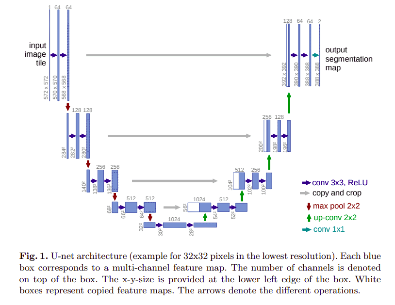
The contracting path consists of two 3 by 3 convolutions which are followed by a rectified linear unit and a 2 by 2 max pooling operation. Downsampling is done by the pooling operation. At each downsampling stage the number of feature channels are doubled. The feature samples are upsampled by the expansive path. Upsampling is followed by a 2 by 2 up-convolution that halves the number of feature channels. The final layer maps the component feature vectors to the needed number of classes. This layer is a 1 by 1 convolution.
The model is trained using the input images, their segmentation maps and a stochastic gradient descent based on Caffe. The full implementation and the trained networks can be found here.
On experimentation, the model achieved a mean intersection-over-union (IOU) of 92%.
IOU is a common metric used to evaluate the performance of object detection and segmentation models. This metric is computed from the ground truth mask and the predicted mask.
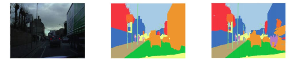
Source. From Left original image, original annotation (ground truth) masks and predicted masks
It basically measures the overlap between the ground truth mask and the predicted mask.
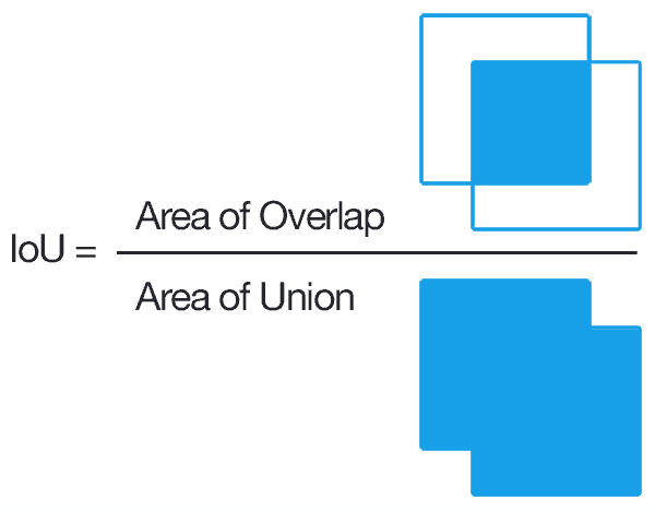
The higher the IOU the better the model’s performance.
FastFCN —Fast Fully-connected network
Since dilated convolutions take a lot of time and memory, this architecture uses a joint upsampling module named Joint Pyramid Upsampling (JPU). The function responsible for extracting high-resolution maps is formulated as a joint upsampling problem. In this method a fully-connected network(FCN) is used as the backbone. The JPU is applied to upsample the low resolution final feature maps. This results in high resolution feature maps.
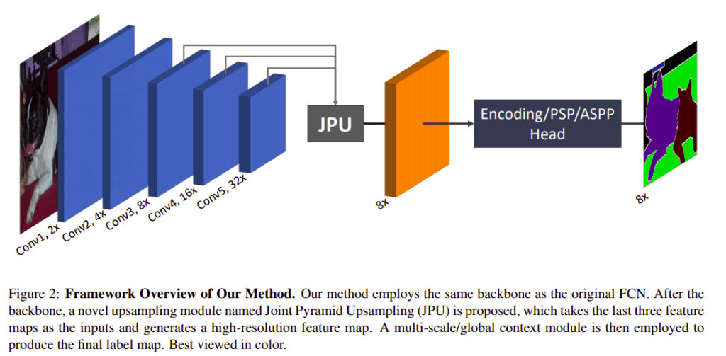
When tested on the Pascal Context dataset, the model achieves a mean Intersection over Union of 53.13%.
The official implementation of this model can be found here.
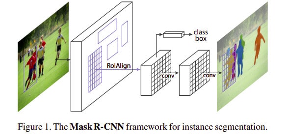
Mask R-CNN
This model is an extension of the Faster R-CNN architecture. The Faster R-CNN is a Fast Region-based Convolutional Network method. It achieves a mean average precision of 66% on PASCAL VOC 2012. Fast R-CNN takes image input inputs coupled with a set of object proposals. It processes the image using a convolutional and max-pooling layer. Thereafter, it produces a convolutional feature map. After this, a fixed layer feature vector is extracted from the feature maps using a region of interest pooling layer. This is done for each region proposal. The feature vectors are fed to fully connected layers that branch into two output layers. Softmax probability estimates over the object classes are produced by one layer. The other layer produces four real-value numbers for every object class. The four describe the position of the bounding box for the objects. In Mask R-CNN, objects are classified and localized using these bounding boxes. The model extends Faster R-CNN via the addition of segmentation masks for each of the regions of interest.
In a later section you will see how the model can be used in Python to segment images.
Weakly- and Semi-Supervised Learning of a Deep Convolutional Network
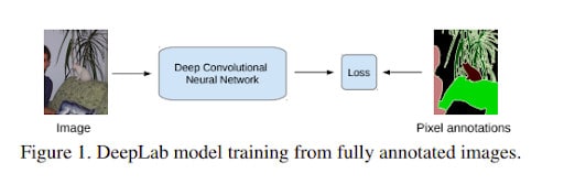
This architecture aims at solving segmentation problems for weakly annotated training images such as bounding boxes or labels. It is also efficient where there are few strongly labeled and many weakly labeled images. The source code for this implementation can be found here. The model achieves a mean intersection-over-union (IOU) score above 70% on the PASCAL VOC segmentation benchmark.
This model uses a combination of Deep Convolutional Neural Networks (DCNN) coupled with a fully connected Conditional Random Field. The combination results in high resolution segmentations. During training, the model requires pixel-level annotated images. Informed by this challenge, the proponents of this model, developed training methods for DCNNs image segmentation models from weak annotations. They also developed new Expectation-Maximization (EM) methods that train DCNN segmentation models on weakly annotated images. The methods they propose switch between estimating latent pixel label and optimization of DCNN parameters by the use stochastic gradient descent (SGD).
DeepLab
This method uses a combination of DCNN and a fully connected Conditional Random Field (CRF). The model achieves a 79.7% mIOU on the PASCAL VOC-2012 semantic image segmentation task. It tackles three major challenges that are encountered when applying DCNN to semantic segmentation:
- reduced feature resolution
- existence of objects at multiple scales
- reduced localization accuracy resulting from DCNN invariance
The model uses atrous convolutions; convolution with upsampled filters. Atrous convolutions enable enlargement of the field of filters without the need to increase the number of parameters or the amount of computation. The existence of objects at multiple scales is solved using atrous spatial pyramid pooling (ASPP).
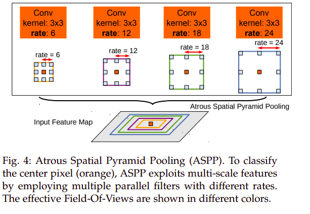
In this method, a feature layer is resampled at multiple rates before convolution happens. This results in capturing of image context at multiple scales. The final problem (reduced localization accuracy resulting from DCNN invariance) is solved by improving the ability of the model to capture fine details via the use of a fully connected Conditional Random Field (CRF). A fully connected pairwise CRF is used because of its ability to capture fine edge details as well as its efficient computation.
Segmentation from Natural Language Expressions
In this paper, the authors focus on the challenge of segmenting an image based on a natural language expression. They propose an end-to-end trainable recurrent and convolutional network model that produces pixel-wise segmentation for the language expression.
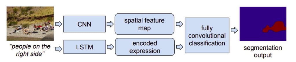
The model jointly learns to process visual and linguistic information. In the model, a recurrent LSTM network is used to encode the expression into a vector representation. Spatial feature maps are extracted from the image using a fully convolutional network. It outputs a spatial response map for the target object.
The model is made up of three components:
- a natural language expression encoder based on a recurrent LSTM
network
- a fully convolutional network that extracts local image descriptors and
generates a spatial feature map
- a fully convolutional classification and upsampling network which takes the encoded expression as input and generates a pixel wise segmentation mask
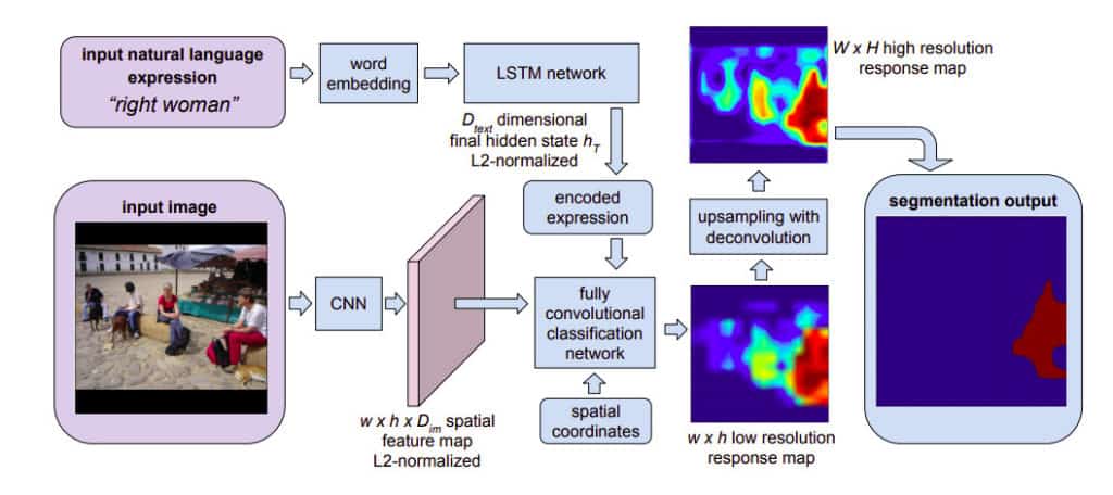
On the ReferIt dataset, the model obtains an overall IoU of 48.03% on high resolution.
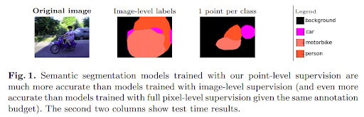
Semantic Segmentation with Point Supervision
The model proposed in this paper is based on humans pointing to objects. It uses a convolutional neural network (CNN) framework for semantic segmentation coupled with point supervision in its training loss function. An objectness prior is also incorporated. Its purpose is to separate objects from the background by using the probability of a pixel belonging to a certain object.
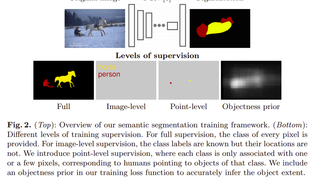
In this approach supervised points are provided on training images. Segmentation on test images is done using the learned model without any additional human input.
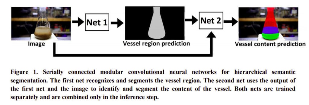
Hierarchical semantic segmentation
Here, Sagi proposes that the task of identifying objects or the contents of a vessel can be viewed as an hierarchical problem. This means that the vessel is first recognized followed by the contents of the vessel. In this case the output of the method that recognizes the vessel is used as input to the method that recognizes the contents of the vessel.
Multiple View Semantic Segmentation
This method proposes a multi-view segmentation framework for images that are captured using a camera that has been mounted on a vehicle driven along streets. It involves laying out a pairwise Markov Random Field (MRF) across multiple views. A graph-based optimization strategy is used to ensure that there are consistent segmentation results across multiple views. Data from Google Street View is used and a new approach for labeling is fronted.
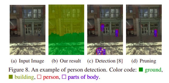
In this method a 3D scene for each sequence with about 100 images is first reconstructed. The user then labels the 3D Points in 3D space. Once the labels of the 3D points are obtained, they can also be used to segment 2D images. That way, one labeling task would give 100 labeled images.
Multi-View Deep Learning for Consistent Semantic Mapping with RGB-D Cameras
This method proposes a strategy for predicting semantic segmentation from RGB-D sequences using a deep neural network. The network is trained to predict multi-view semantics in a self-supervised manner.
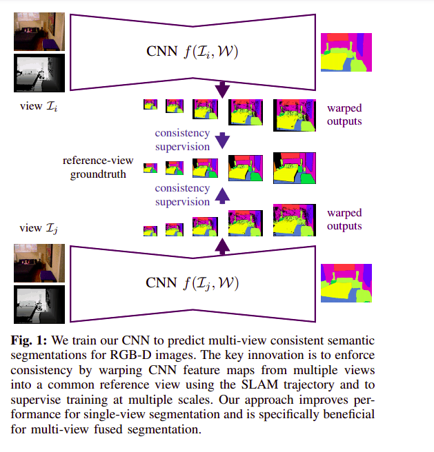
As seen above the CNN is regularized with multiview consistency constraints. RGBD simultaneous localization and mapping (SLAM) is used to warp the network outputs of multiple frames into the reference view with ground truth annotation. Predictions that are obtained from the network are aggregated into keyframes so as to increase the segmentation accuracy during testing.
Here is the architecture for that semantic segmentation CNN.
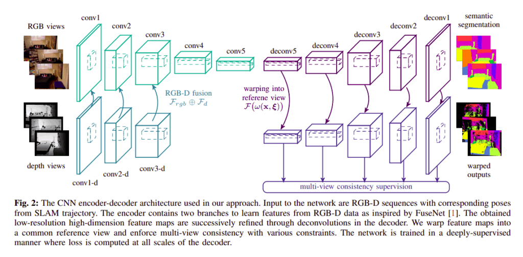
The encoder-decoder CNN is based on FuseNet. It is improved by incorporating multi-scale loss minimization which leads to better segmentation performance. The encoder uses convolutional layers to extract a hierarchy of features. It also aggregates spatial information via pooling layers. This increases the receptive field. Finally, the encoder generates low resolution high dimensional feature maps that are upsampled to the input resolution by the encoder. This is done using layers of memorized unpooling and deconvolution.
Advanced Image Segmentation Loss Functions
Apart from the classic cross-categorical entropy loss function, there are other advanced loss functions that you can use in semantic segmentation.
Distribution-based Loss
In traditional machine learning loss functions were based on the distribution of labels. As an example, the categorical cross entropy is derived from the Multinoulli distribution.
Weighted Binary Cross-Entropy
This loss function is a variant of the cross-entropy loss function where positive examples are weighted by a given coefficient. It is therefore useful in scenarios involving imbalance classes.
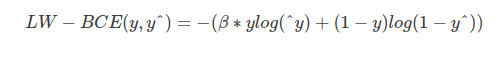
β is used for tuning the false positives and the false negatives. For example setting β greater than 1 reduces the number of false negatives.
Balanced Cross-Entropy
In Balanced cross entropy (BCE) loss the positive and negative samples are both weighted.
Focal Loss
In this function, the role of easy examples is down weighted while the contribution of hard examples is magnified. In doing so, the training is focused on hard examples. It is a great choice for highly imbalanced problems.
Region-based Loss
Let’s now switch gears and look at region based loss functions.
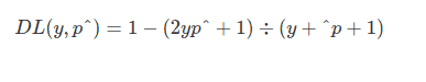
Dice Loss
This loss function is computed from the Dice coefficient. This coefficient is a metric that is used to compute the similarity between two images.
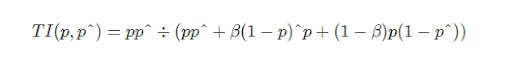
Tversky Loss
The Tversky Loss is a variant of the Dice Loss that uses a β coefficient to add weight to false positives and false negatives.
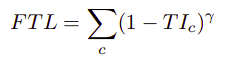
Focal Tversky Loss
Focal Tversky loss aims at learning hard examples aided by the γ coefficient that ranges from 1 to 3.
Sensitivity Specificity Loss
This loss deals with the problem of class imbalance using the w parameter.
Log-Cosh Dice Loss
Log-Cosh Dice Loss is a variant of Dice Loss that is inspired by log-cosh for smoothing. It is used in datasets that are skewed.
Boundary-based Loss
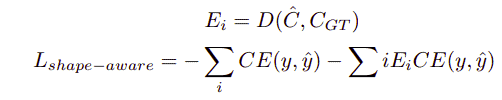
Shape-aware Loss
Shape-aware loss computes the average point to curve Euclidean distance among curves of the predicted segmentation to the ground truth. It then uses this as a coefficient to the cross-entropy loss function. It is majorly used in boundaries that are hard to segment.
Hausdorff Distance Loss (HD)
This loss is based on the Hausdorff Distance metric. The loss tackles the non-convex nature of the Hausdorff Distance in order to make it usable in segmentation models.
Compounded Loss
Combo Loss
The combo loss is a combination of the weighted sum of Dice loss and the Binary Cross-Entropy. It aims at incorporating Dice’s class balancing and the curve smoothing of cross-entropy.
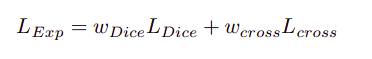
Exponential Logarithmic Loss
This loss uses a combination of Dice loss and Cross-entropy loss aimed at focusing on less accurately predicted cases.
Data Augmentation for Semantic Segmentation
One of the main problems faced in computer vision is not having enough data. Usually very little data will lead to poor model performance. Collecting more data is not always possible, for example in medical diagnosis as mentioned earlier. This problem is addressed via creating more training data from the existing data. This process is known as image augmentation. Some of the techniques used to create more training data for semantic segmentation include:
- flipping the images e.g vertical and horizontal flips
- rotating the images
- adding contrast to the image
- adjusting the brightness of the image
- implementing cropping e.g random cropping
- using a combination of these strategies
just to mention a few.
Some of these strategies can be applied natively in most deep learning frameworks. However, there are libraries that are focused on augmentations. One such package is Albumentations. Some of the transformations supported by the package include Posterize, Solarize, and Sharpen.
Image Segmentation on the Edge
While image segmentation models work seamlessly on the browser, they can not be directly deployed on edge devices such as mobile devices. For example, a TensorFlow model has to be converted to a format that can be deployed to a mobile device; i.e the TF Lite format. TensorFlow Lite is bundled with a set of tools that enable the deployment of image segmentation models on mobile, embedded, and IoT devices. TF Lite allows for fast inference since the segmentation models are small enough to fit on an edge device. Once you have your TensorFlow segmentation model you can easily convert it to the TF Lite format using the TensorFlow Lite converter. Alternatively you can use pre-trained models that are provided by Google’s ML Kit or Fritz AI.
Image Segmentation in Python
As mentioned earlier, you will now get a chance to see the Mask R-CNN model in action. In this article, you will use Matterport’s implementation. It will produce bounding boxes and segmentation masks for the objects that have been detected in an image. Since the project contains MS COCO pre-trained weights, training the model from scratch won’t be necessary.
`os` will be used to set the path to the root directory, `skimage` for image processing and `matplotlib` for visualizing the image. This image will be used for this segmentation work.
import os
import sys
import skimage.io
import matplotlib
import matplotlib.pyplot as plt
ROOT_DIR = os.path.abspath("./")
The next step is to import Mask R-CNN.
sys.path.append(ROOT_DIR)
from mrcnn import utils
import mrcnn.model as modellib
from mrcnn import visualize
After this, import the MS COCO configuration and set the path where the trained model and logs will be stored.
If the COCO weights are not available, you will need to download them.
if not os.path.exists(COCO_MODEL_PATH):
    utils.download_trained_weights(COCO_MODEL_PATH)
Next set the path to the folder containing the image that you want to segment.
IMAGE_DIR = os.path.join(ROOT_DIR, "images") Since you are using one image, set a batch size of one to the COCO config.
class InferenceConfig(coco.CocoConfig):
    GPU_COUNT = 1
    IMAGES_PER_GPU = 1
config = InferenceConfig()
You can use `config.display()` to view all the configurations.
At this point, the model can be instantiated. The mode is set to inference because you are just making predictions. While at it, you also need to load the COCO weights that were downloaded earlier.
model = modellib.MaskRCNN(mode="inference", model_dir=MODEL_DIR, config=config)
model.load_weights(COCO_MODEL_PATH, by_name=True)
You then need to create a list of the 81 classes that are available from COCO.
class_names = ['BG', 'person', 'bicycle', 'car', 'motorcycle', 'airplane',
               'bus', 'train', 'truck', 'boat', 'traffic light',
               'fire hydrant', 'stop sign', 'parking meter', 'bench', 'bird',
               'cat', 'dog', 'horse', 'sheep', 'cow', 'elephant', 'bear',
               'zebra', 'giraffe', 'backpack', 'umbrella', 'handbag', 'tie',
               'suitcase', 'frisbee', 'skis', 'snowboard', 'sports ball',
               'kite', 'baseball bat', 'baseball glove', 'skateboard',
               'surfboard', 'tennis racket', 'bottle', 'wine glass', 'cup',
               'fork', 'knife', 'spoon', 'bowl', 'banana', 'apple',
               'sandwich', 'orange', 'broccoli', 'carrot', 'hot dog', 'pizza',
               'donut', 'cake', 'chair', 'couch', 'potted plant', 'bed',
               'dining table', 'toilet', 'tv', 'laptop', 'mouse', 'remote',
               'keyboard', 'cell phone', 'microwave', 'oven', 'toaster',
               'sink', 'refrigerator', 'book', 'clock', 'vase', 'scissors',
               'teddy bear', 'hair drier', 'toothbrush']
Now use `skimage` to process the image that you will run the segmentation on.
image = skimage.io.imread(os.path.join(IMAGE_DIR, image.jpg'))
Obtaining the results can be done using the models `detect` method.
results = model.detect([image], verbose=1) Now visualize the results using the `display_instances` function.
r = results[0]
visualize.display_instances(image, r['rois'], r['masks'], r['class_ids'],
class_names, r['scores']) 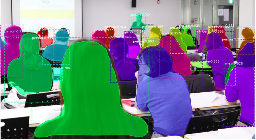
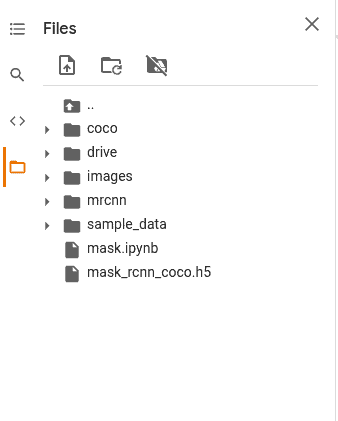
The entire source code for this implementation can be found here. A Google Colab implementation can be found here. For the Colab implementation to work, you will need to download the Mask R-CNN code from Github and upload it to Colab as shown below.
Conclusion
In this article you have covered so much ground as far as image segmentation is concerned. Specifically you have learned:
- What image segmentation is
- The difference between image segmentation vs. instance segmentation
- Various image segmentation architectures
- Loss functions that are specific to image segmentation
- Data augmentation for image segmentation
Now go forth and explore the image segmentation use case mentioned here, as well as more.