
In this article, you are going to learn about the special type of Neural Network known as “Long Short Term Memory” or LSTMs. This article is divided into 4 main parts.
- What is Sequential Data?
- Importance of LSTMs (What are the restrictions with traditional neural networks and how LSTM has overcome them) .
In this section, you’ll learn about traditional Neural Networks, and Recurrent Neural Networks and their shortcomings, and go over how LSTMs or Long Short Term Memory have overcome those shortcomings. - Mathematical Intuition of LSTMs
- Practical Implementation in PyTorch
What is Sequential data?
If you work as a data science professional, you may already know that LSTMs are good for sequential tasks where the data is in a sequential format. Let’s begin by understanding what sequential data is.
In layman’s terms, sequential data is data which is in a sequence. In other words, it is a kind of data where the order of the data matters. Let’s look at some of the common types of sequential data with examples.
1. Language data/a sentence
For example “My name is Ahmad”, or “I am playing football”. In these kinds of examples, you can not change the order to “Name is my Ahmad”, because the correct order is critical to the meaning of the sentence.
2.Time Series Data
For example, the Stock Market price of Company A per year. In this kind of data, you have to check it year by year and to find a sequence and trends – you can not change the order of the years.
3.Biological Data
For example, a DNA sequence must remain in order.
If you observe, sequential data is everywhere around us, for example, you can see audio as a sequence of sound waves, textual data, etc. These are some common examples of sequential data that must preserve its order. Experiments over time have proven that traditional neural networks, such as dense neural networks, are not good for these tasks and are unable to preserve the sequence. Thus, you’ll need some kind of architecture that can preserve the sequence of the data.
The next section will go over the limitations in traditional neural network architectures, as well as some problems in Recurrent Neural Networks, which will build on the understanding of LSTMs.
Importance of LSTMs
To grasp the concept and importance of LSTM, you’ll need to understand why we need LSTM. What are the limitations of other Neural Network architectures that made us feel that we need another architecture that is suitable for processing Sequential Data.
For this, you’ll also need to understand the working and shortcomings of Recurrent Neural Networks (RNN), as LSTM is a modified architecture of RNN. Don’t worry if you do not know much about Recurrent Neural Networks, this article will discuss their structure in greater detail later.
Problems with Traditional Neural Network
To begin, let’s look at the image below to understand the working of a simple neural network.
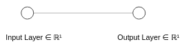
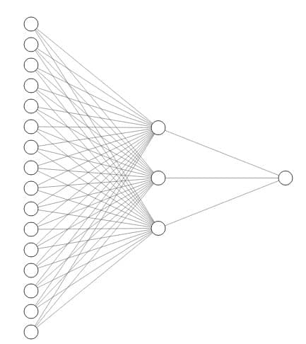
This image shows the working of a simple neural network where X is the input and ŷ is the output created via mathematical calculations. This is a simple One-to-One Neural Network. You can similarly have a many to many neural network or a densely connected neural network as shown in the image below
While these networks perform better than traditional machine learning algorithms, they have several shortcomings. One of which, is of course sequential data. Other shortcomings of traditional neural networks are:
- They have a fixed input length
- They can not remember the sequence of the data, i.e order is not important
- Can not share parameters across the sequence
Let’s have a brief look at these problems, then dig deeper into RNN.
The first problem discussed here is that they have a fixed input length, which means that the neural network must receive an input that is of equal length. Now for a normal sequential data set, such as the GDP of a country per year, this issue is not a big deal as they have the same number of features. But this problem arises when dealing with data such as language, where each sentence is of different length. For example
[“Hello”, “How”, “are”, “you] is a vector with length 4 and [“My”, “Name”, “is”, “Ahmad”, “and”, “I”, “am”, “sleeping”] is a vector having 9 words. This is a serious problem that is very limiting. While Scientists have discovered some workarounds in a normal neural network, they don’t perform as well for high level models.
The second limitation with traditional neural networks is that they can not remember the sequence of the data, or the order is not important to them. Let’s understand this problem with an example.
Let’s say you have 1 sentence that is “I am Ahmad, not Hassan”, and another sentence, that is “I am Hassan, not Ahmad”. A traditional neural network would deal with these sentences the same, because both sentences have the same words. Though, we know that in this case the order is very important and completely changes the meaning of the words.
Another example of this problem is shown in this figure.

Credits: MIT 6.S191 Intro to Deep Learning
Now the third limitation with traditional neural networks is that they do not share the parameter across the sequence. So, to understand this problem let’s take the sentence “what is your name? My name is Ahmad”. Now you’ll want the network to deal with the common word as the same. In this case “name” should have shared parameters, and the neural network should be able to tell how many times “name” appears in a single sequence. Unfortunately, a traditional neural network does not recognize this type of pattern which makes it unsuited for particular machine learning solutions.
As you can see, these limitations make a simple neural network unfit for sequential tasks. This is especially limiting when dealing with language-related tasks, or tasks that have a variable input.
Now let’s look at some of the important requirements that are mandatory for sequential tasks.
- The model should be able to handle variable-length sequences
- Can track Long term dependencies (Will discuss later on)
- Maintain information about the order
- Share parameters across the sequence.
Now let’s discuss RNN, or Recurrent Neural Networks. RNN was originally designed to fulfill the requirements that traditional neural networks could not.
What is a Recurrent Neural Network?
RNN or recurrent neural networks, originally were designed to handle some of the shortcomings that traditional neural networks have when dealing with sequential data.
Let’s compare the structure of a Recurrent Neural Network, to a simple Neural Network.
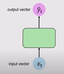
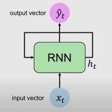
Simple Neural Network
VS
RNN
Here you can see that the Simple Neural Network is unidirectional, which means it has a single direction, whereas the RNN, has loops inside it to persist the information over timestamp t. This is the reason RNN’s are known as “recurrent” neural networks. This looping preserves the information over the sequence. Now, let’s dig deeper to understand what is happening under the hood.
A simplified explanation is that there has been a recurrence relation applied at every timestamp to process a sequence.
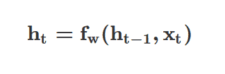
Where ht is the current cell state, fw is a function that is parameterized by weights, ht-1 is the previous or last state, and Xt is the input vector at timestamp t. An important thing to note here is that you are using the same function and set of parameters at every timestamp.
Now that it is not ignoring the previous timestamps (or order of the sequence), you are able to keep them in check via ht-1 which is the previous timestamp that helps update the current timestamp.
Now let’s deep dive a little bit further.
Given the input vector, Xt, RNN applies a function to update its hidden state which is a standard Neural Network operation.
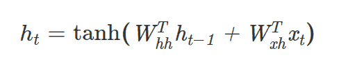
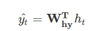
As you can see in the equation above, you feed in both input vector Xt and the previous state ht-1 into the function. Here you’ll have 2 separate weight matrices then apply the Non-linearity (tanh) to the sum of input Xt and previous state ht-1 after multiplication to these 2 weight matrices. Finally, you’ll have the output vector ŷt at the timestamp t.
The above function is a modified, transformed version of this internal state, which results simply by multiplication by another weight matrix. This is simply how RNN can update its hidden state and calculate the output.
Let’s unroll the RNN loop overtime to get an even better understanding. The figure below will give you a better picture of how you can unfold the loop inside the RNN.
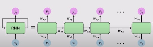
Unfolding RNNs, Credits: MIT 6S191
Above, you can see that you are adding the input at every time stamp, and generating the output ŷ at every timestamp. As mentioned earlier, you are going to use the same weight matrices at every timestamp. And, just as a reminder, Whh is the weight matrix by which you update the previous state, as shown in the equation above, and as visible in the figure. Wxh is the weight matrix that is applied at every timestamp to the input value. Why is the weight matrix that is applied to the output ŷ
From these outputs ŷ0, ŷ1, ŷ2, …., ŷt, you can calculate the Loss L1, L2, …, Lt, at each timestamp t. This will complete the forward pass or forward propagation and completes the section of RNN. Let’s now do a quick recap of the working of RNN.
- RNN updates the hidden state via input and previous state
- Compute the output matrix via a simple neural network operation that is W x h
- Return the output and update the hidden state
You can combine, and take the sum of all these losses to calculate a total loss L, through which you can propagate backwards to complete the backpropagation. Below is a visual representation of how backpropagation in RNN works.
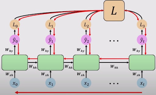
Backpropagation in RNNs, Credits: MIT 68191
Backpropagation in RNNs work similarly to backpropagation in Simple Neural Networks, which has the following main steps.
- Feed Forward Pass
- Take the derivative of the loss with each parameter
- Shift parameters to update the weights and minimize the Loss.
If you look closely at the figure above, you can see that it runs similarly to a simple Neural Network. It completes a feedforward pass, calculates the loss at each output, takes the derivative of each output, and propagates backward to update the weights. Since errors are calculated and are backpropagated at each timestamp, this is also known as “backpropagation through time”.
Computing the gradients require a lot of factors of Whh plus repeated gradient computations, which makes it a bit problematic. There are 2 main problems that can arise in an RNN, which LSTM helps solve:
- Exploding Gradients
- Vanishing Gradients
Exploding Gradients is a problem when many of the values, that are involved in the repeated gradient computations (such as weight matrix, or gradient themselves), are greater than 1, then this problem is known as an Exploding Gradient. In this problem, gradients become extremely large, and it is very hard to optimize them. This problem can be solved via a process known as Gradient Clipping, which essentially scales back the gradient to smaller values.
Vanishing Gradients occur when many of the values that are involved in the repeated gradient computations (such as weight matrix, or gradient themselves) are too small or less than 1. In this problem, gradients become smaller and smaller as these computations occur repeatedly. This can be a major problem. Let’s look at an example.
Let’s say you have a word prediction problem that you would like to solve, “The clouds are in the ____”. Now since this is not a long sequence, the RNN can easily remember this, and the weights associated with each word (each word is input at timestamp) are not too big nor too small. But, when you have a large sequence, for example,
“My name is Ahmad, I live in Pakistan, I am a good boy, I am in 5th grade, I am _____”. Now for the RNN to predict the word “Pakistani” here, it has to remember the word Pakistan, but since it is a very long sequence, and there are vanishing gradients, i.e very minimal weights for the word “Pakistan”, so the model will have a difficult time predicting the word “Pakistani” here. This is also known as the problem of long term dependency.
Now you can see why having small values of calculations (vanishing gradients) is such a big problem.
This problem can be solved in 3 ways:.
- Activation Function (ReLU instead of tanh)
- Weights initialization
- Changing Network Architecture
This section will focus on the 3rd solution that is changing the network architecture. In this solution, you modify the architecture of RNNs and use the more complex recurrent unit with Gates such as LSTMs or GRUs (Gated Recurrent Units). GRUs are out of scope for this article so we will dive only into LSTMs in-depth.
Long Short Term Memory (LSTMs)
LSTMs are a special type of Neural Networks that perform similarly to Recurrent Neural Networks, but run better than RNNs, and further solve some of the important shortcomings of RNNs for long term dependencies, and vanishing gradients. LSTMs are best suited for long term dependencies, and you will see later how they overcome the problem of vanishing gradients.
The main idea behind LSTM is that they have introduced self-looping to produce paths where gradients can flow for a long duration (meaning gradients will not vanish). This idea is the main contribution of initial long-short-term memory (Hochireiter and Schmidhuber, 1997). Later on, a crucial addition has been made to make the weight on this self-loop conditioned on the context, rather than fixed. This can help in changing the time scale of integration. This means that even when LSTM has fixed parameters, the time scale of integration can change based on the input sequence because the time constants are outputs by the model itself.
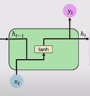
Let’s have a quick recap of a single block of RNN.
- Single Computation layer with tanh activation
- ht is the function of the previous cell state ht-1 and current input Xt as shown in the above equations.
Below is the workflow of a single RNN cell.
Let’s now focus on LSTM blocks. LSTM modules contain computational blocks that control information flow. These involve more complexity, and more computations compared to RNNs. But as a result, LSTM can hold or track the information through many timestamps. In this architecture, there are not one, but two hidden states.
In LSTM, there are different interacting layers. These layers interact to selectively control the flow of information through the cell.
The key building block behind LSTM is a structure known as gates. Information is added or removed through these gates. Gates can optionally let information through, for example via a sigmoid layer, and pointwise multiplication, as shown in the figure below.
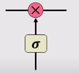
A gate consists of a neural net layer, like a sigmoid, and a pointwise multiplication shown in red in the figure above. Sigmoid is forcing the input between 0 and 1, which determines how much information is captured when passed through the gate, and how much is retained when it passes through the gate. For example, 0 means no information is retained, and 1 means all information is retained.
Let’s dive more into the working of LSTMs.
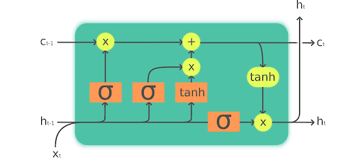
Image Credits Fast.ai
How LSTM works in 4 simple steps:
1. Forget the irreverent history
This is done through the forget gate. The main purpose of the forget gate is to decide which information the LSTM should keep or carry, and which information it should throw away. This is the function of the prior internal state ht-1 and the new input Xt.
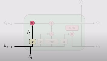
This happens because not all the information in a sequence or a sentence needs to be important. Some information is relatively more important, and some information is not important at all. For example: “My name is Ahmad”. In this sentence, the important information for LSTM to store is that the name of the person speaking the sentence is “Ahmad”. But a sentence can also have a piece of irrelevant information such as “My friend’s name is Ali. He is a good boy. He’s in fourth grade. My father is sleeping. Ali is a sharp and intelligent boy.” Here you can see that it’s talking about “Ali”, and has an irrelevant sentence about my father. This is an example where LSTM can decide what relevant information to send, and what not to send.
This forget gate is denoted by fi(t) (for time step t and cell i), which sets this weight value between 0 and 1 which decides how much information to send, as discussed above. Let’s look at the equation.
Where x(t) is the current input vector, h(t) is the current hidden state, containing the outputs of all the LSTM cells, and bf, Uf, Wf are respectively biases, input weights, and recurrent weights for the forget gates.
2. Perform the computations & store the relevant new information
When LSTM has decided what relevant information to keep, and what to discard, it then performs some computations to store the new information. These computations are performed via the input gate or sometimes known as an external input gate. To update the internal cell state, you have to do some computations before. First you’ll pass the previous hidden state, and the current input with the bias into a sigmoid activation function, that decides which values to update by transforming them between 0 and 1.
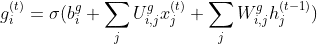
3. Use these 2 steps to selectively update their internal state
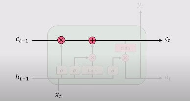
Since there is now enough information, this time in order to update its internal state, you’ll have conditional self-loop weight f(i)t. First, we do the pointwise multiplication of the previous cell state sit-1 by the forget vector (or gate), then take the output from the input gate git and add it. Then we perform simple neural network operations.
Where b, U, and W respectively denote the biases, input weights, and the recurrent weights into the LSTM cells. You will see that this internal state is also denoted as ct, as shown in the figure below from MIT Deep Learning Class.
4. Output Gate
Lastly, you’ll have the output via the output gate. This output gate controls what information is to be coded into the cell state sent to the network as input in the next timestamp. This hidden state (which is sent to the next network) is also used for predictions. It works as follows. You pass the newly modified state that you get from step 3 to the tanh function. Then multiply the output with the sigmoid output of a standard neural network operation performed on previous outputs and input at the current timestamp. The output is denoted by hit
The equations are as follows:
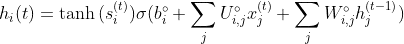
Graphically, you can see it from this picture, taken from the MIT Deep Learning Course, freely available on YouTube.
An essential property of LSTM is that the gating and updating mechanisms work to create the internal Cell state Ct or St which allow uninterrupted gradient workflow over time. You can think of this as a highway of cell states where gradients can flow uninterrupted. This enables us to eliminate the Vanishing Gradient problems, as shown in standard or vanilla RNN.
Variants on Long-Short Term Memory
There are different variants of Long Short Term Memory, and the one I have explained is quite common. Not all of the LSTMs are like the above example, and you will find some difference in mathematical equations and the working of the LSTM cells. The differences are not major differences though, and if you understand them clearly, you can understand them easily too.
Here is a graphical depiction of a basic LSTM structure to help give a deeper understanding of the concepts defined above.
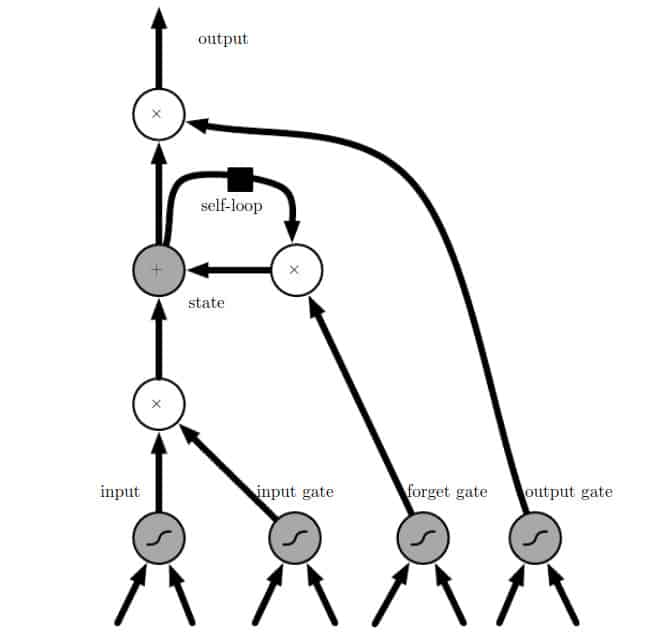
1 Block of LSTM: Credits Deep Learning Book
Let’s now have a quick recap of the key concepts of LSTM.
1. LSTM can maintain a separate cell state from what they are outputting
2. They use gates to control the flow of information
3. Forget Gate is used to get rid of useless information
4. Store relevant information from the current input
5. Selectively update the cell state
Output Gate returns the filtered version of the cell state
Backpropagation over time with uninterrupted gradient flow
Backpropagation in LSTMs work similarly to how it was described in the RNN section.

Back Propagation in RNN
Next, take the sum of total losses, add them up, and flow backward over time. If you want to get a mathematical derivative process, I refer you to this article and an upgraded version of the same article here. They have done a wonderful job in calculating all the mathematical derivatives necessary for backpropagation.
Practical Implementation in PyTorch
Let’s look at a real example of Starbucks’ stock market price, which is an example of Sequential Data. In this example we will go over a simple LSTM model using Python and PyTorch to predict the Volume of Starbucks’ stock price.
Let’s load the dataset first. You can download the dataset from this link. You can load it using pandas.
import numpy as np |
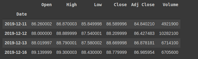
You can check the head of the dataset via
df.head(5) |
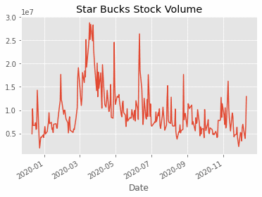
Now, you can plot the label column, with the timeframe to check the original trend of the volume of stock.
plt.style.use(‘ggplot’) |
Since this article is more focused on the PyTorch part, we won’t dive in to further data exploration and simply dive in on how to build the LSTM model. Before making the model, one last thing you have to do is to prepare the data for the model. This is also known as data-preprocessing.
Let’s get the data and the labels separate from a single dataframe.
X = df.iloc[:, :-1]
y = df.iloc[:, 5:6]
Since this is not an article focused on different techniques of data preprocessing, you will use StandardScaler for the features, and MinMaxScaler (to scale values between 0 and 1) for the output values. Notice that it is a regression problem, so it is very beneficial to scale your outputs otherwise you will be dealing with a huge loss.
from sklearn.preprocessing import StandardScaler, MinMaxScaler
mm = MinMaxScaler()
ss = StandardScaler()


X_ss = ss.fit_transform(X)
y_mm = mm.fit_transform(y)
This will transform and scale the dataset. The next thing is splitting the dataset into 2 parts. 1 is for the training, and the other part is for testing the values. Since it is sequential data, and order is important, you will take the first 200 rows for training, and 53 for testing the data. You will notice that you can make a really good prediction on such a low amount of data using LSTMs.
#first 200 for training

X_train = X_ss[:200, :]
X_test = X_ss[200:, :]

y_train = y_mm[:200, :]
y_test = y_mm[200:, :]
Next, you can print out the training and testing data shapes for the confirmation.
print("Training Shape", X_train.shape, y_train.shape)
print("Testing Shape", X_test.shape, y_test.shape) 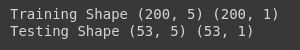
If you are programming in PyTorch for a while, you should know that in PyTorch, all you deal with are tensors, which you can think of as a powerful version of numpy. So you have to convert the dataset into tensors.
Let’s import important libraries first.
import torch #pytorch
import torch.nn as nn
from torch.autograd import Variable
You can simply convert the Numpy Arrays to Tensors and to Variables (which can be differentiated) via this simple code.
X_train_tensors = Variable(torch.Tensor(X_train))
X_test_tensors = Variable(torch.Tensor(X_test))

y_train_tensors = Variable(torch.Tensor(y_train))
y_test_tensors = Variable(torch.Tensor(y_test))
Now the next step is to check the input format of an LSTM. This means that since LSTM is specially built for sequential data, it can not take in simple 2-D data as input. They need to have the timestamp information with them too, as we discussed that we need to have input at each timestamp. So let’s convert the dataset.
#reshaping to rows, timestamps, features

X_train_tensors_final = torch.reshape(X_train_tensors,   (X_train_tensors.shape[0], 1, X_train_tensors.shape[1]))


X_test_tensors_final = torch.reshape(X_test_tensors,  (X_test_tensors.shape[0], 1, X_test_tensors.shape[1]))
Now you can confirm the shape of the dataset via printing the shapes.
print("Training Shape", X_train_tensors_final.shape, y_train_tensors.shape)
print("Testing Shape", X_test_tensors_final.shape, y_test_tensors.shape) 
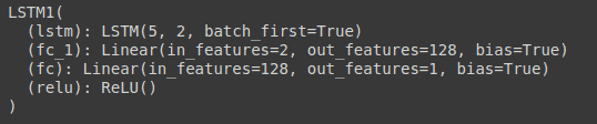
Now, you are good to go, and it’s time to build the LSTM model. Since PyTorch is way more pythonic, every model in it needs to be inherited from nn.Module superclass.
Here you’ve defined all the important variables, and layers. Next you are going to use 2 LSTM layers with the same hyperparameters stacked over each other (via hidden_size), you have defined the 2 Fully Connected layers, the ReLU layer, and some helper variables. Next, you are going to define the forward pass of the LSTM.
class LSTM1(nn.Module):
    def __init__(self, num_classes, input_size, hidden_size, num_layers, seq_length):
        super(LSTM1, self).__init__()
        self.num_classes = num_classes #number of classes
        self.num_layers = num_layers #number of layers
        self.input_size = input_size #input size
        self.hidden_size = hidden_size #hidden state
        self.seq_length = seq_length #sequence length

        self.lstm = nn.LSTM(input_size=input_size, hidden_size=hidden_size,
                          num_layers=num_layers, batch_first=True) #lstm
        self.fc_1 =  nn.Linear(hidden_size, 128) #fully connected 1
        self.fc = nn.Linear(128, num_classes) #fully connected last layer

        self.relu = nn.ReLU()

    def forward(self,x):
        h_0 = Variable(torch.zeros(self.num_layers, x.size(0), self.hidden_size)) #hidden state
        c_0 = Variable(torch.zeros(self.num_layers, x.size(0), self.hidden_size)) #internal state
        # Propagate input through LSTM
        output, (hn, cn) = self.lstm(x, (h_0, c_0)) #lstm with input, hidden, and internal state
        hn = hn.view(-1, self.hidden_size) #reshaping the data for Dense layer next
        out = self.relu(hn)
        out = self.fc_1(out) #first Dense
        out = self.relu(out) #relu
        out = self.fc(out) #Final Output
        return out
Here you have defined the hidden state, and internal state first, initialized with zeros. First of all, you are going to pass the hidden state and internal state in LSTM, along with the input at the current timestamp t. This will return a new hidden state, current state, and output. You’ll reshape the output so that it can pass to a Dense Layer. Next, simply apply activations, and pass them to the dense layers, and return the output.
This completes the Forward Pass and the class LSTM1. You will apply backpropagation logic while training the model at runtime.
You can see the model statistics via printing the model.
Let’s define some important variables now, that you will use. These are hyperparameters, such as the number of epochs, hidden size, etc.
num_epochs = 1000 #1000 epochs
learning_rate = 0.001 #0.001 lr

input_size = 5 #number of features
hidden_size = 2 #number of features in hidden state
num_layers = 1 #number of stacked lstm layers

num_classes = 1 #number of output classes
Now you will instantiate the class LSTM1 object.
lstm1 = LSTM1(num_classes, input_size, hidden_size, num_layers, X_train_tensors_final.shape[1]) #our lstm class Let’s define the Loss function and optimizer.
criterion = torch.nn.MSELoss()    # mean-squared error for regression
optimizer = torch.optim.Adam(lstm1.parameters(), lr=learning_rate)
Now loop for the number of epochs, do the forward pass, calculate the loss, improve the weights via the optimizer step.# Train the model
for epoch in range(num_epochs):
  outputs = lstm1.forward(X_train_tensors_final) #forward pass
  optimizer.zero_grad() #caluclate the gradient, manually setting to 0

  # obtain the loss function
  loss = criterion(outputs, y_train_tensors)

  loss.backward() #calculates the loss of the loss function

  optimizer.step() #improve from loss, i.e backprop
  if epoch % 100 == 0:
    print("Epoch: %d, loss: %1.5f" % (epoch, loss.item()))
This will start the training for 1000 epochs, and print the loss at every 100 epoch.
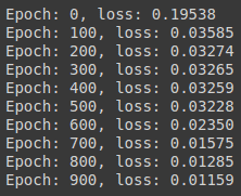
You can see that there is less loss, which means it is performing well. Let’s plot the predictions on the data set, to check out how it’s performing.
But before performing predictions on the whole dataset, you’ll need to bring the original dataset into the model suitable format, which can be done by using similar code as above.
df_X_ss = ss.transform(df.iloc[:, :-1]) #old transformers
df_y_mm = mm.transform(df.iloc[:, -1:]) #old transformers

df_X_ss = Variable(torch.Tensor(df_X_ss)) #converting to Tensors
df_y_mm = Variable(torch.Tensor(df_y_mm))
#reshaping the dataset
df_X_ss = torch.reshape(df_X_ss, (df_X_ss.shape[0], 1, df_X_ss.shape[1]))
You can now simply perform predictions on the whole dataset via a forward pass, and then to plot them, you will convert the predictions to numpy, reverse transform them (remember that you transformed the labels to check the actual answer, and that you’ll need to reverse transform it) and then plot it.
train_predict = lstm1(df_X_ss)#forward pass
data_predict = train_predict.data.numpy() #numpy conversion
dataY_plot = df_y_mm.data.numpy()

data_predict = mm.inverse_transform(data_predict) #reverse transformation
dataY_plot = mm.inverse_transform(dataY_plot)
plt.figure(figsize=(10,6)) #plotting
plt.axvline(x=200, c='r', linestyle='--') #size of the training set

plt.plot(dataY_plot, label='Actuall Data') #actual plot
plt.plot(data_predict, label='Predicted Data') #predicted plot
plt.title('Time-Series Prediction')
plt.legend()
plt.show()
And you can see the predictions
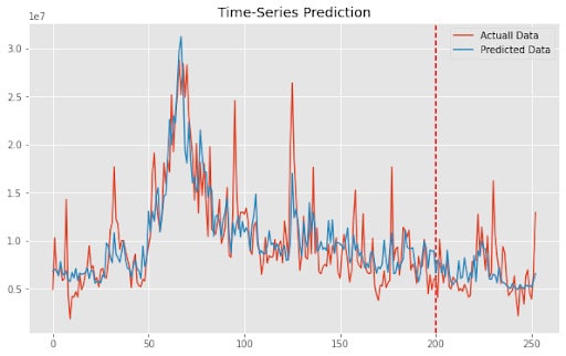
You can see that the model is performing quite well despite using a smaller dataset.
Learning Outcomes:
Here’s a recap of what you’ve learned in this article:
- What is Sequential Data?
- Why Traditional Models are not good for Sequential Data
- How does RNN work?
- What are the shortcomings of RNNs?
- What are LSTM and how do they work?
- How LSTM solves the problems of RNN
- Practical coding of LSTMs in PyTorch
Hopefully this article can help expand the types of problems you can solve as a data science team, and will develop your skills to become a more valuable data scientist.
References: