
In this article, there is an in-depth discussion on
- What are Loss Functions
- What are Evaluation Metrics?
- Commonly used Loss functions in Keras (Regression and Classification)
- Built-in loss functions in Keras
- What is the custom loss function?
- Implementation of common loss functions in Keras
- Custom Loss Function for Layers i.e Custom Regularization Loss
- Dealing with NaN values in Keras Loss
- Why should you use a Custom Loss?
- Monitoring Keras Loss using callbacks
What are Loss Functions
Loss functions are one of the core parts of a machine learning model. If you’ve been in the field of data science for some time, you must have heard it. Loss functions, also known as cost functions, are special types of functions, which help us minimize the error, and reach as close as possible to the expected output.
In deep learning, the loss is computed to get the gradients for the model weights and update those weights accordingly using backpropagation.
Source: FreeCodeCamp
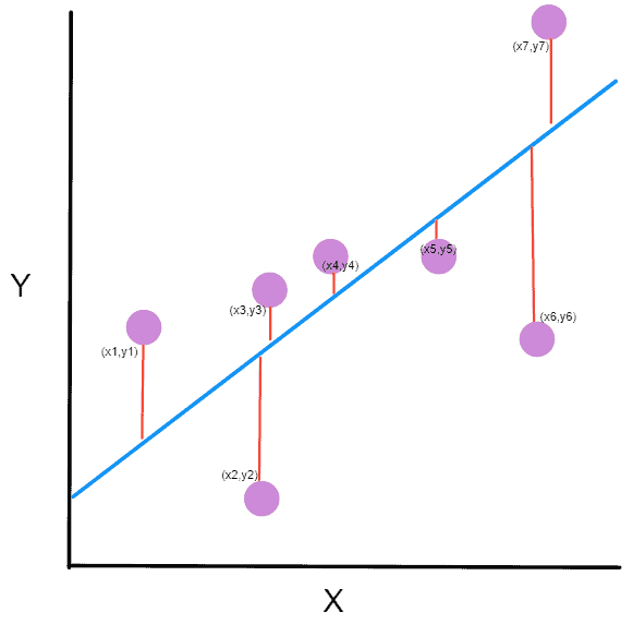
Basic working or understanding of error can be gained from the image above, where there is an actual value and a predicted value. The difference between the actual value and predicted value can be known as error.
This can be written in the equation form as

So our goal is to minimize the difference between the predicted value which is hθ(x) and the actual value y. In other words, you have to minimize the value of the cost function. This main idea can be understood better from the following picture by Professor Andrew NG where he explains that choosing the correct value of θ0 and θ1 which are weights of a model, such that our prediction hθ is closest to y which is the actual output.
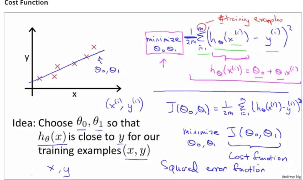
Here Professor Andrew NG is using the Mean Squared Error function, which will be discussed later on.
An easy explanation can be said that the goal of a machine learning model is to minimize the cost and maximize the evaluation metric. This can be achieved by updating the weights of a machine learning model using some algorithm such as Gradient Descent.
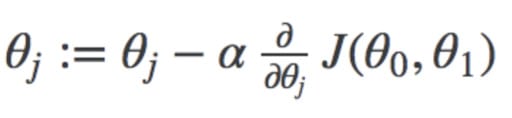
Here you can see the weight that is being updated and the cost function, that is used to update the weight of a machine learning model.
What are Evaluation Metrics
Evaluation metrics are the metrics used to evaluate and judge the performance of a machine learning model. Evaluating a machine learning project is very essential. There are different types of evaluation metrics such as ‘Mean Squared Error’, ‘Accuracy’, ‘Mean Absolute Error’ etc. The cost functions used, such as mean squared error, or binary cross-entropy are also metrics, but they are difficult to read and interpret how our model is performing. So there is a need for other metrics like Accuracy, Precision, Recall, etc. Using different metrics is important because a model may perform well using one measurement from one evaluation metric, but may perform poorly using another measurement from another evaluation metric.
Here you can see the performance of our model using 2 metrics. The first one is Loss and the second one is accuracy. It can be seen that our loss function (which was cross-entropy in this example) has a value of 0.4474 which is difficult to interpret whether it is a good loss or not, but it can be seen from the accuracy that currently it has an accuracy of 80%.
Hence it is important to use different evaluation metrics other than loss/cost function only to properly evaluate the model’s performance and capabilities.
Some of the common evaluation metrics include:
- Accuracy
- Precision
- Recall
- F-1 Score
- MSE
- MAE
- Confusion Matrix
- Logarithmic Loss
- ROC curve
And many more.
Commonly Used Loss Functions in Machine Learning Algorithms and their Keras Implementation
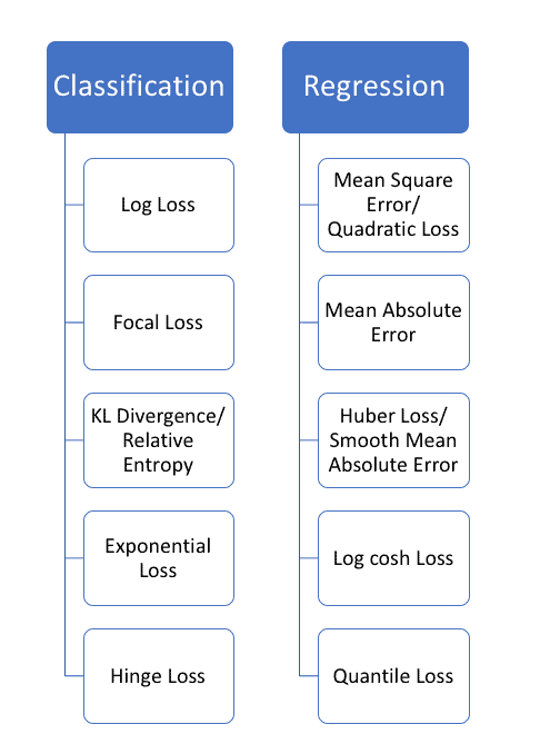
Source: Heartbeat
Common Regression Losses:
Regression is the type of problem where you are going to predict a continuous variable. This means that our variable can be any number, not some specific labels.
For example, when you have to predict prices of houses, it can be a house of any price, so it is a regression problem.
Some of the common examples of regressions tasks are
- Prices Prediction
- Stock Market Prediction
- Financial Forecasting
- Trend Analysis
- Time Series Predictions
And many more.
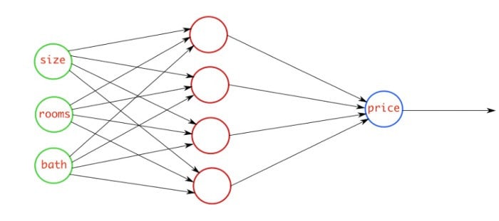
This figure above explains the regression problem where you are going to predict the price of the house by checking three features which are size of the house, rooms in the house, and baths in the house. Our model will check these features, and will predict a continuous number that will be the price of the house.
Since regression problems deal with predicting a continuous number, so you have to use different types of loss then classification problems. Some of the commonly used loss functions in regression problems are as follows.
Mean Squared Error
Mean squared error, also known as L2 Loss is mainly used for Regression Tasks. As the name suggests, it is calculated by taking the mean of the square of the loss/error which is the difference between actual and predicted value.
The Mathematical equation for Mean Squared Error is
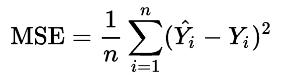
Where Ŷi is the predicted value, and Yi is the actual value. Mean Squared Error penalizes the model for making errors by taking the square. This is the reason that this loss function is less robust to outliers in the dataset.
Implementation in Keras.
Standalone Usage:
					import keras
import numpy as np

y_true = np.array([[10.0,7.0]]) #sample data
y_pred = np.array([[8.0, 6.0]])

a = keras.losses.MSE(y_true, y_pred)

print(f'Value of Mean Squared Error is {a.numpy()}')
Here predicted values and the true values are passed inside the Mean Squared Error Object from keras.losses and computed the loss. It returns a tf.Tensor object which has been converted into numpy to see more clearly.
Using via compile Method:
Keras losses can be specified for a deep learning model using the compile method from keras.Model..
					model = keras.Sequential([
                     keras.layers.Dense(10, input_shape=(1,), activation='relu'),
                     keras.layers.Dense(1)

])
And now the compile method can be used to specify the loss and metrics.
model.compile(loss='mse', optimizer='adam')
Now when our model is going to be trained, it will use the Mean Squared Error loss function to compute the loss, update the weights using ADAM optimizer.
model.fit(np.array([[10.0],[20.0], [30.0],[40.0],[50.0],[60.0],[10.0], [20.0]]), np.array([6, 12, 18,24,30, 36,6, 12]), epochs=10)
Mean Absolute Error
Mean Absolute error, also known as L1 Error, is defined as the average of the absolute differences between the actual value and the predicted value. This is the average of the absolute difference between the predicted and the actual value.
Mathematically, it can be shown as:
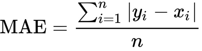
The Mean Absolute error uses the scale-dependent accuracy measure which means that it uses the same scale which is being used by the data being measured, thus it can not be used in making comparisons between series that are using different scales.
Mean Squared Error is also a common regression loss, which means that it is used to predict a continuous variable.
Standalone Implementation in Keras:
					import keras
import numpy as np


y_true = np.array([[10.0,7.0]]) #dummy data
y_pred = np.array([[8.0, 6.0]])

c = keras.losses.MAE(y_true, y_pred) #calculating loss

print(f'Value of Mean Absolute Error is {c.numpy()}')
What you have to do is to create an MAE object from keras.losses and pass in our true and predicted labels to calculate the loss using the equation given above.
Implementing using compile method
When working with a deep learning model in Keras, you have to define the model structure first.
					model = keras.models.Sequential([
                                   keras.layers.Dense(10, input_shape=(1,), activation='relu'),
                                   keras.layers.Dense(1)
])
After defining the model architecture, you have to compile it and use the MAE loss function. Notice that either there is linear or no activation function in the last layer means that you are going to predict a continuous variable.
model.compile(loss='mae', optimizer='adam')
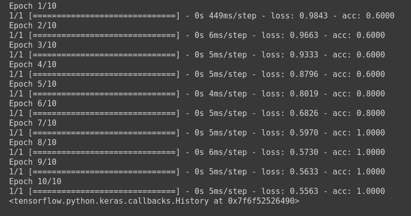
You can now simply just fit the model to check our model’s progress. Here our model is going to train on a very small dummy random array just to check the progress.
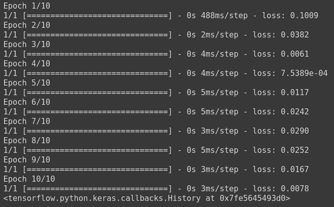
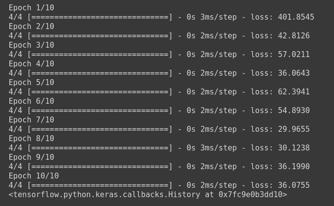
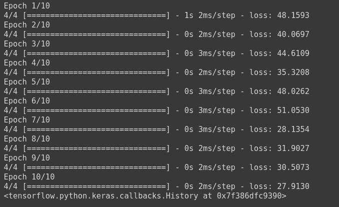
model.fit(np.array([[10.0],[20.0], [30.0],[40.0],[50.0],[60.0],[10.0], [20.0]]), np.array([6, 12, 18,24,30, 36,6, 12]), epochs=10)
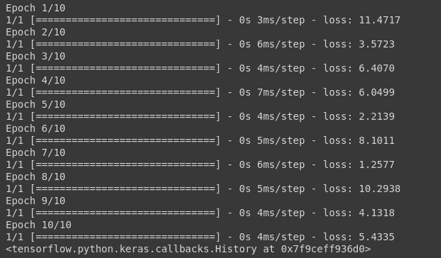
And you can see the loss value which has been calculated using the MAE formula for each epoch.
Common Classification Losses:
Classification problems are those problems, in which you have to predict a label. This means that the output should be only from the given labels that you have provided to the model.
For example: There is a problem where you have to detect if the input image belongs to any given class such as dog, cat, or horse. The model will predict 3 numbers ranging from 0 to 1 and the one with the highest probability will be picked
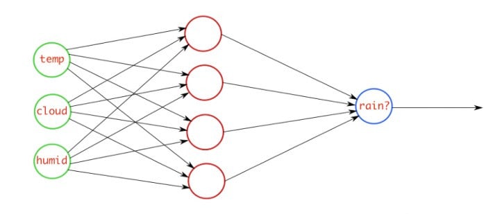
If you want to predict whether it is going to rain tomorrow or not, this means that the model can output between 0 and 1, and you will choose the option of rain if it is greater than 0.5, and no rain if it is less than 0.5.
Common Classification Loss:
1. Cross-Entropy
Cross Entropy is one of the most commonly used classification loss functions. You can say that it is the measure of the degrees of the dissimilarity between two probabilistic distributions. For example, in the task of predicting whether it will rain tomorrow or not, there are two distributions, one for True, and one for False.
Cross Entropy is of 3 main types.
a. Binary Cross Entropy
Binary Cross Entropy, as the name suggests, is the cross entropy that occurs between two classes, or in the problem of binary classification where you have to detect whether it belongs to class ‘A’, and if it does not belong to class ‘A’, then it belongs to class ‘B’.
Just like in the example of rain prediction, if it is going to rain tomorrow, then it belongs to rain class, and if there is less probability of rain tomorrow, then this means that it belongs to no rain class.
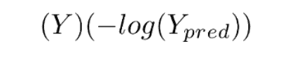
Mathematical Equation for Binary Cross Entropy is

This loss function has 2 parts. If our actual label is 1, the equation after ‘+’ becomes 0 because 1-1 = 0. So loss when our label is 1 is
And when our label is 0, then the first part becomes 0. So our loss in that case would be
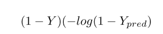
This loss function is also known as the Log Loss function, because of the logarithm of the loss.
Standalone Implementation:
You can create an object for Binary Cross Entropy from Keras.losses. Then you have to pass in our true and predicted labels.
					import keras
import numpy as np

y_true=np.array([[1.0]])
y_pred = np.array([[0.9]])

loss = keras.losses.BinaryCrossentropy()
print(f"BCE LOSS VALUE IS {loss(y_true, y_pred).numpy()}")
Implementation using compile method
To use Binary Cross Entropy in a deep learning model, design the architecture, and compile the model while specifying the loss as Binary Cross Entropy.
import keras
import numpy as np
model = keras.models.Sequential([
keras.layers.Dense(16, input_shape=(2,), activation='relu'),
keras.layers.Dense(8, activation='relu'),
keras.layers.Dense(1, activation='sigmoid') #Sigmoid for probabilistic distribution
])
model.compile(optimizer='sgd', loss=keras.losses.BinaryCrossentropy(), metrics=['acc'])# binary cross entropy
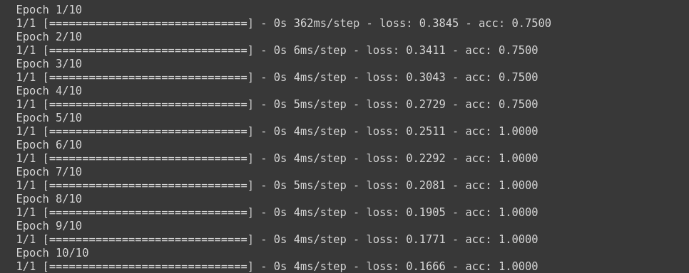
model.fit(np.array([[10.0, 20.0],[20.0,30.0],[30.0,6.0], [8.0, 20.0]]),np.array([1,1,0,1]) ,epochs=10)
This will train the model using Binary Cross Entropy Loss function.
b. Categorical Cross Entropy
Categorical Cross Entropy is the cross entropy that is used for multi-class classification. This means for a single training example, you have n probabilities, and you take the class with maximum probability where n is number of classes.

Mathematically, you can write it as:

This double sum is over the N number of examples and C categories. The term 1yi ∈ Cc shows that the ith observation belongs to the cth category. The Pmodel[yi ∈ Cc] is the probability predicted by the model for the ith observation to belong to the cth category. When there are more than 2 probabilities, the neural network outputs a vector of C probabilities, with each probability belonging to each class. When the number of categories is just two, the neural network outputs a single probability ŷi , with the other one being 1 minus the output. This is why the binary cross entropy looks a bit different from categorical cross entropy, despite being a special case of it.
Standalone Implementation
You will create a Categorical Cross Entropy object from keras.losses and pass in our true and predicted labels, on which it will calculate the Cross Entropy and return a Tensor.
Note that you have to provide a matrix that is one hot encoded showing probability for each class, as shown in this example.
					import keras
import numpy as np

y_true = [[0, 1, 0], [0, 0, 1]] #3classes

y_pred = [[0.05, 0.95, 0], [0.1, 0.5, 0.4]]


loss = keras.losses.CategoricalCrossentropy()
print(f"CCE LOSS VALUE IS {loss(y_true, y_pred).numpy()}")
Implementation using compile method
When implemented using the compile method, you have to design a model in Keras, and compile it using Categorical Cross Entropy loss. Now when the model is trained, it is calculating the loss based on categorical cross entropy, and updating the weights according to the given optimizer.
import keras
import numpy as np
from keras.utils import to_categorical #to one hot encode the data
model = keras.models.Sequential([
keras.layers.Dense(16, input_shape=(2,), activation='relu'),
keras.layers.Dense(8, activation='relu'),
keras.layers.Dense(3, activation='softmax') #Softmax for multiclass probability
])
model.compile(optimizer='sgd', loss=keras.losses.CategoricalCrossentropy(), metrics=['acc'])# categorical cross entropy
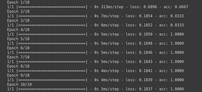
model.fit(np.array([[10.0, 20.0],[20.0,30.0],[30.0,6.0], [8.0, 20.0], [-1.0, -100.0], [-10.0, -200.0]]) ,to_categorical(np.array([1,1,0,1, 2, 2])) ,epochs=10)
Here, it will train the model on our dummy dataset.
c. Sparse Categorical Cross Entropy
Mathematically, there is no difference between Categorical Cross Entropy, and Sparse Categorical Cross Entropy according to official documentation. Use this cross entropy loss function when there are two or more label classes. We expect labels to be provided as integers. If you want to provide labels using one-hot representation, please use CategoricalCrossentrop loss. There should be # classes floating point values per feature for y_pred and a single floating point value per feature for y_true.“
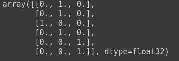
As you have seen earlier in Categorical Cross Entropy that one hot matrix has been passed as the true labels, and predicted labels. An example of which is as follows:
to_categorical(np.array([1,1,0,1, 2, 2]))
For using sparse categorical cross entropy in Keras, you need to pass in the label encoded labels. You can use sklearn for this purpose.
Lets see this example to understand better.
					from sklearn.preprocessing import LabelEncoder

le = LabelEncoder()
output = le.fit_transform(np.array(['High chance of Rain', 'No Rain', 'Maybe', 'Maybe', 'No Rain', 'High chance of Rain']))
Here a LabelEncoder object has been created, and the fit_transform method is used to encode it. The output of it is as follows.
Standalone Implementation
To perform standalone implementation, you need to perform label encoding on labels. There should be n floating point values per feature for each true label, where n is the total number of classes.
					from sklearn.preprocessing import LabelEncoder
t = LabelEncoder()
y_pred = [[0.1,0.1,0.8], [0.1,0.4,0.5], [0.5,0.3,0.2], [0.6,0.3,0.1]]
y_true = t.fit_transform(['Rain', 'Rain', 'High Changes of Rain', 'No Rain'])
loss = keras.losses.SparseCategoricalCrossentropy()
print(f"Sparse Categorical Loss is {loss(y_true, y_pred).numpy()} ")
Implementation using model.compile
To implement Sparse Categorical Cross Entropy in a deep learning model, you have to design the model, and compile it using the loss sparse categorical cross entropy. Remember to perform label encoding of your class labels so that sparse categorical cross entropy can work.
					import keras
import numpy as np
from sklearn.preprocessing import LabelEncoder
model = keras.models.Sequential([
                                   keras.layers.Dense(16, input_shape=(2,), activation='relu'),
                                   keras.layers.Dense(8, activation='relu'),
                                   keras.layers.Dense(3, activation='softmax') #Softmax for multiclass probability
])
le = LabelEncoder()
model.compile(optimizer='sgd', loss=keras.losses.SparseCategoricalCrossentropy(), metrics=['acc'])# sparse categorical cross entropy
Now the model will be trained on the dummy dataset.
model.fit(np.array([[10.0, 20.0],[20.0,30.0],[30.0,6.0], [8.0, 20.0], [-1.0, -100.0], [-10.0, -200.0]]) ,le.fit_transform(np.array(['High chance of Rain', 'High chance of Rain', 'High chance of Rain', 'Maybe', 'No Rain', 'No Rain'])) ,epochs=10)
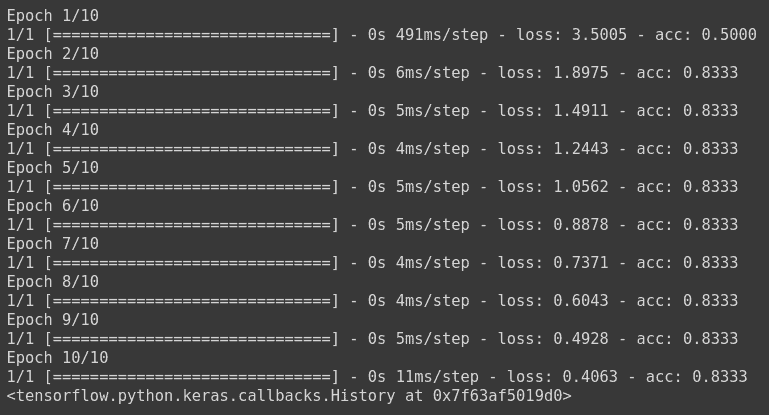
The model has been trained, where the loss is calculated using sparse categorical cross entropy, and the weights have been updated using stochastic gradient descent.
2. Hinge Loss
Hinge loss is a commonly used loss function for classification problems. It is mainly used in problems where you have to do ‘maximum-margin’ classification. A common example of which is Support Vector Machines.
The following image shows how maximum margin classification works.
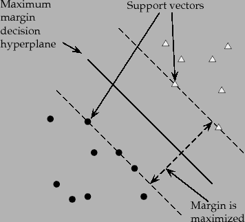
Source: Stanford NLP Group
The mathematical formula for hinge loss is:
Where yi is the actual label and ŷ is the predicted label. When prediction is positive, value goes on one side, and when the prediction is negative, value goes totally opposite. This is why it is known as maximum margin classification.
Standalone Implementation:
To perform standalone implementation of Hinge Loss in Keras, you are going to use Hinge Loss Class from keras.losses.
					import keras
import numpy as np
y_true = [[0., 1.], [0., 0.]]
y_pred = [[0.6, 0.4], [0.4, 0.6]]
h = keras.losses.Hinge()
print(f'Value for Hinge Loss is {h(y_true, y_pred).numpy()}')
Implementation using compile Method
To implement Hinge loss using compile method, you will design our model and compile it where you will mention our loss as Hinge.
Note that Hinge Loss works best with tanh as the activation in the last layer.
					import keras
import numpy as np
					model = keras.models.Sequential([
                                   keras.layers.Dense(16, input_shape=(2,), activation='relu'),
                                   keras.layers.Dense(8, activation='tanh'),
                                   keras.layers.Dense(1, activation='tanh')
])
model.compile(optimizer='adam', loss=keras.losses.Hinge(), metrics=['acc'])# Hinge Loss
					from sklearn.preprocessing import LabelEncoder

le = LabelEncoder()
model.fit(np.array([[10.0, 20.0],[20.0,30.0],[30.0,6.0], [-1.0, -100.0], [-10.0, -200.0]]) ,le.fit_transform(np.array(['High chance of Rain', 'High chance of Rain', 'High chance of Rain', 'No Rain', 'No Rain'])) ,epochs=10, batch_size=5)
This will train the model using Hinge Loss and update the weights using Adam optimizer.
Custom Loss Functions
So far you have seen some of the important cost functions that are widely used in industry and are good and easy to understand, and are built-in by famous deep learning frameworks such as Keras, or PyTorch. These built-in loss functions are enough for most of the typical tasks such as classification, or regression.
But there are some tasks, which can not be performed well using these built-in loss functions, and require some other loss that is more suitable for that task. For that purpose, a custom loss function is designed that calculates the error between the predicted value and actual value based on custom criteria.
Why you should use Custom Loss
Artificial Intelligence in general and Deep Learning in general is a very strong research field. There are various industries using Deep Learning to solve complex scenarios.
There is a lot of research on how to perform a specific task using Deep Learning. For example there is a task on generating different recipes of food using the picture of the food. Now on papers with code (a famous site for deep learning and machine learning research papers), there are a lot of research papers on this topic.

Now Imagine you are reading a research paper where the researchers thought that using Cross Entropy, or Mean Squared Error, or whatever the general loss function is for that specific type of the problem is not good enough. It may require you to modify it according to the need. This may involve adding some new parameters, or a whole new technique to achieve better results.
Now when you are implementing that problem, or you hired some data scientists to solve that specific problem for you, you may find that this specific problem is best solved using that specific loss function which is not available by default in Keras, and you need to implement it yourself.
A custom loss function can improve the models performance significantly, and can be really useful in solving some specific problems.
To create a custom loss, you have to take care of some rules.
- The loss function must only take two values, that are true labels, and predicted labels. This is because in order to calculate the error in prediction, these two values are needed. These arguments are passed from the model itself when the model is being fitted.
For example:
					def customLoss(y_true, y_pred):
            	return loss
	model.compile(loss=customLoss, optimizer='sgd')
2. Make sure that you are making the use of y_pred or predicted value in the loss function, because if you do not do so, the gradient expression would not be defined, and it can throw some error.
3. You can now simply use it in model.compile function just like you would use any other loss function.
Example:
Let’s say you want to perform a regression task where you want to use a custom loss function that divides the loss value of Mean Squared Error by 10. Mathematically, it can be denoted as:
Now to implement it in Keras, you need to define a custom loss function, with two parameters that are true and predicted values. Then you will perform mathematical functions as per our algorithm, and return the loss value.
Note that Keras Backend functions and Tensorflow mathematical operations will be used instead of numpy functions to avoid some silly errors. Keras backend functions work similarly to numpy functions.
					import keras
import numpy as np
from tensorflow.python.ops import math_ops

def custom_loss(y_true, y_pred):
 diff = math_ops.squared_difference(y_pred, y_true)  #squared difference
 loss = K.mean(diff, axis=-1) #mean over last dimension
 loss = loss / 10.0
 return loss
Here you can see a custom function with 2 parameters that are true and predicted values, and the first step was to calculate the squared difference between the predicted labels and the true labels using squared difference function from Tensorflow Python ops. Then the mean is calculated to complete the mean squared error, and divided by 10 to complete our algorithm. The loss value is then returned.
You can use it in our deep learning model, by compiling our model and setting the loss function to the custom loss defined above.
					model = keras.Sequential([
                   keras.layers.Dense(10, activation='relu', input_shape=(1,)),
                   keras.layers.Dense(1)
])

model.compile(loss=custom_loss, optimizer='sgd')

X_train = np.array([[10.0],[20.0], [30.0],[40.0],[50.0],[60.0],[10.0], [20.0]])
y_train = np.array([6.0, 12, 18,24,30, 36,6, 12]) #dummy data

model.fit(X_train, y_train, batch_size=2, epochs=10)
Passing multiple arguments to a Keras Loss Function
Now, if you want to add some extra parameters to our loss function, for example, in the above formula, the MSE is being divided by 10. Now if you want to divide it by any value that is given by the user, you need to create a Wrapper Function with those extra parameters.
Wrapper function in short is a function whose job is to call another function, with little or no computation. The additional parameters will be passed in the wrapper function, while the main 2 parameters will remain the same in our original function.
Let’s see it with the code.
					def wrapper(param1):
 def custom_loss_1(y_true, y_pred):
   diff = math_ops.squared_difference(y_pred, y_true)  #squared difference
   loss = K.mean(diff, axis=-1) #mean
   loss = loss / param1
   return loss
 return custom_loss_1
To do the standalone computation using Keras, You will first create the object of our wrapper, and then pass in it y_true and y_pred parameters.
					loss = wrapper(10.0)

final_loss = loss(y_true=[[10.0,7.0]], y_pred=[[8.0, 6.0]])
print(f"Final Loss is {final_loss.numpy()}")
You can use it in our deep learning models by simply calling the function by using appropriate value for our param1.
					model1 = keras.Sequential([
                   keras.layers.Dense(10, activation='relu', input_shape=(1,)),
                   keras.layers.Dense(1)
])

model1.compile(loss=wrapper(10.0), optimizer='sgd')
Here the model has been compiled using the value 10.0 for our param1.
The model can be trained and the results can be seen .
model1.fit(X_train, y_train, batch_size=2, epochs=10)
Creating Custom Loss for Layers
Loss functions that are applied to the output of the model (i.e what you have seen till now) are not the only way to calculate and compute the losses. The custom losses for custom layers or subclassed models can be computed for the quantities which you want to minimize during the training like the regularization losses.
These losses are added using add_loss() function from keras.Layer.
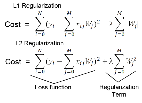
For example, if you want to add custom l2 regularization in our layer, the mathematical formula of which is as follows:
You can create your own custom regularizer class which should be inherited from keras.layers..
					from keras.layers import Layer
from tensorflow.math import reduce_sum, square

class MyActivityRegularizer(Layer):

    def __init__(self, rate=1e-2):
        super(MyActivityRegularizer, self).__init__()
        self.rate = rate

    def call(self, inputs):
        self.add_loss(self.rate * reduce_sum(square(inputs)))
        return inputs
Now, since the regularized loss has been defined, you can simply add it in any built-in layer, or create our own layer.
class SparseMLP(Layer):
  """Stack of Linear layers with our custom regularization loss."""

  def __init__(self, output_dim):
      super(SparseMLP, self).__init__()
      self.dense_1 = layers.Dense(32, activation=tf.nn.relu)
      self.regularization = MyActivityRegularizer(1e-2)
      self.dense_2 = layers.Dense(output_dim)

  def call(self, inputs):
      x = self.dense_1(inputs)
      x = self.regularization(x)
      return self.dense_2(x)
Here custom sparse MLP layer has been defined, where when stacking two linear layers, The custom loss function has been added which will regularize the weights of our deep learning model.
It can be tested:
					mlp = SparseMLP(1)
y = mlp(np.random.normal(size=(10, 10)))

print(mlp.losses)  # List containing one float32 scalar
It returns a tf.Tensor, which can be converted into numpy using mlp.losses.numpy() method.
Dealing with NaN in Custom Loss in Keras
There are many reasons that our loss function in Keras gives NaN values. If you are new to Keras or practical deep learning, this could be very annoying because you have no idea why Keras is not giving the desired output. Since Keras is a high level API, built over low level frameworks such as Theano, Tensorflow etc. it is difficult to know the problem.
There are many different reasons for which many people have received NaN in their loss, like shown in this figure below
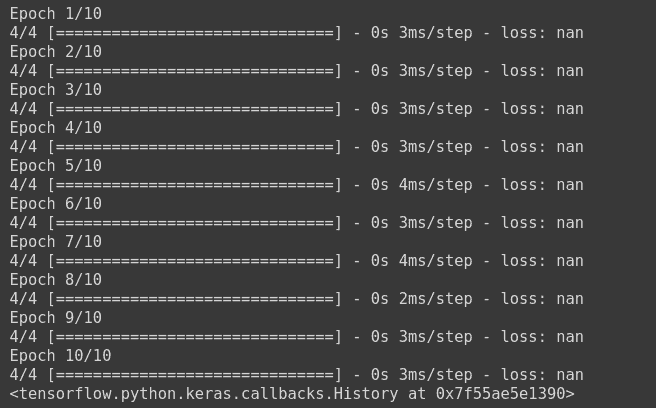
Some of the main reasons, which are very common, are as follows:
1. Missing Values in training dataset
This is one of the most common reasons for why the loss is nan while training. You should remove all the missing values from your dataset, or fill them using a good strategy, such as filling with mean. You can check nan values by using Pandas built in functions.
print(np.any(np.isnan(X_test)))
And if there are any null values, you can either use pandas fillna() function to fill them, or dropna() function to drop those values.
2. Loss is unable to get traction on training dataset
This means that the custom loss function you designed, is not suitable for the dataset, and the business problem you are trying to solve. You should look at the problem from another perspective, and try to find a suitable loss function for your problem.
3. Exploding Gradients
Exploding Gradients is a very common problem especially in large neural networks where the value of your gradients become very large. This problem can be solved using Gradient Clipping.
In Keras, you can add gradient clipping to your model when compiling it by adding a parameterclipnorm=x in the selected choice of optimizer. This will clip all the gradients above the value x.
For example:
opt = keras.optimizers.Adam(clipnorm=1.0)
This will clip all the gradients that are greater than 1.0. You can add it into your model as
model.compile(loss=custom_loss, optimizer=opt)
Using RMSProp optimizer function with heavy regularization also helps in diminishing the exploding gradients problem.
4. Dataset is not scaled
Scaling and normalizing the dataset is important. Unscaled data can lead the neural network to behave very strangely. Hence it is advised to properly scale the data.
There are 2 most commonly used scaling methods, and both of them are easily implementable in sklearn which is a famous Machine Learning Library in Python.
- StandardScaler
					from sklearn.preprocessing import StandardScaler
ss = StandardScaler()

X_train_scale = ss.fit_transform(X_train) #using fit_transform so that it can fit on data, and other data can be normalized to same scale
X_test_scale = ss.transform(X_test) #using trasnfrom to get it on same scale as training
2. MinMax Scaler
					from sklearn.preprocessing import StandardScaler
ss = StandardScaler()

X_train_scale = ss.fit_transform(X_train) #using fit_transform so that it can fit on data, and other data can be normalized to same scale
X_test_scale = ss.transform(X_test) #using trasnfrom to get it on same scale as training
5. Dying ReLU problem
A dead ReLU happens, when the relu function always outputs the same value (0 mostly). This means that it takes no role in the discrimination between the inputs. Once a ReLU reaches this state, it is unrecoverable because the function gradient at 0 is also 0, so gradient descent will not change the weights and the model will not improve.
This can be improved by using the Leaky ReLU activation function, where there is a small positive gradient for negative inputs. y=0.01x when x < 0 say
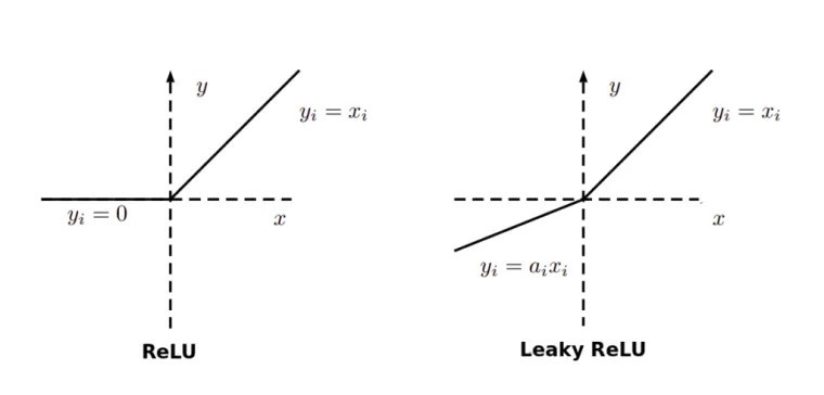
Hence, it is advised to use Leaky ReLU to avoid NaNs in your loss.
In Keras, you can add a leaky relu layer as follows.
keras.layers.LeakyReLU(alpha=0.3, **kwargs)
6. Not a good choice of optimizer function
If you are using Stochastic Gradient Descent, then it is very likely that you are going to face the exploding gradients problem. One way to tackle it is by Scheduling Learning Rate after some epochs, but now due to more advancements and research it has been proven that using a per-parameter adaptive learning rate algorithm like Adam optimizer, you no longer need to schedule the learning rate.
So there are chances that you are not using the right optimizer function.
To use the ADAM optimizer function in Keras, you can use it from keras.optimizers class.
					keras.optimizers.Adam(
    learning_rate=0.001,
    beta_1=0.9,
    beta_2=0.999,
    epsilon=1e-07,
    amsgrad=False,
    name="Adam",
    **kwargs
)
model.compile(optimizer= keras.optimizers.Adam(), loss=custom_loss)
7. Wrong Activation Function
The wrong choice of activation function can also lead to very strange behaviour of the deep learning model. For example if you are working on a multi-class classification problem, and using the relu activation function or sigmoid activation function in the final layer instead of categorical_crossentropy loss function, that can lead the deep learning model to perform very weirdly.
8. Low Batch Size
It has been seen that the optimizer functions on a very low batch size such as 16 or 32 are less stable, as compared to the batch size of 64 or 128.
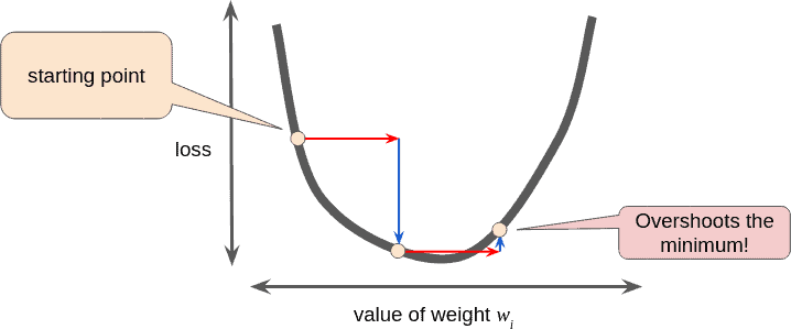
9. High Learning Rate
High learning rate can lead the deep learning model to not converge to optimum, and it can get lost somewhere in between.
Hence it is advisable to use a lower amount of Learning Rate. It can also be improved using Hyper Parameter Tuning.
10. Different file type (for NLP Problems)
If you are doing some textual problem, you can check your file type by running the following command.
Linux
$ file -i {input}
OSX
$ file -I {input}
This will give you the file type. If that file type is ISO-8859-1 or us-ascii then try converting the file to utf-8 or utf-16le.
Monitoring Keras Loss using Callbacks
It is important to monitor your loss when you are training the model, so that you can understand different types of behaviours your model is showing. There are many callbacks introduced by Keras using which you can monitor the loss. Some of the famous ones are:
1. CSVLogger
CSVLogger is a callback provided by Keras that can be used to save the epoch result in a csv file, so that later on it can be visualized, information could be extracted, and the results of epochs can be stored.
You can use CSVLogger from keras.callbacks.
					from keras.callbacks import CSVLogger

csv_logger = CSVLogger('training.csv')
model.fit(X_train, Y_train, callbacks=[csv_logger])
This will fit the model on the dataset, and stores the callback information in a training.csv file, which you can load in a dataframe and visualize it.
2. TerminateOnNaN
Imagine you set the training limit of your model to 1000 epochs, and your model starts showing NaN loss. You can not just sit and stare at the screen while the progress is 0. Keras provides a TerminateOnNan callback that terminates the training whenever NaN loss is encountered.
					import keras
terNan = keras.callbacks.TerminateOnNaN()
model.fit(X_train, Y_train, callbacks=[terNan])
3. RemoteMonitor
RemoteMonitor is a powerful callback in Keras, which can help us monitor, and visualize the learning in real time.
To use this callback, you need to clone hualos by Francis Chollet, who is the creator of Keras.
					git clone https://github.com/fchollet/hualos
cd hualos
python api.py
Now you can access the hualos at localhost:9000 from your browser. Now you have to define the callback, and add it to your model while training
					monitor = RemoteMonitor()
hist = model.fit( train_X, train_Y, nb_epoch=50, callbacks=[ monitor ] )
During the training, the localhost:9000 is automatically updated, and you can see the visualizations of learning in real time.
4. EarlyStopping
EarlyStopping is a very useful callback provided by Keras, where you can stop the training earlier than expected based on some monitor value.
For example you set your epochs to be 100, and your model is not improving after the 10th epoch. You can not sit and stare at the screen so that model may finish the training, and you can change the architecture of the model. Keras provides EarlyStopping callback, which is used to stop the training based on some criteria.
es = keras.callbacks.EarlyStopping(
    monitor="val_loss",
    patience=3,
)
Here, the EarlyStopping callback has been defined, and the monitor has been set to the validation loss value. And it will check that if the value of validation loss does not improve for 3 epochs, it will stop the training.
This article should give you good foundations in dealing with loss functions, especially in Keras, implementing your own custom loss functions which you develop yourself or a researcher has already developed, and you are implementing that, their implementation using Keras a deep learning framework, avoiding silly errors such as repeating NaNs in your loss function, and how you should monitor your loss function in Keras.
Hopefully, now you have a good grip on these topics:
- What are Loss Functions
- What are Evaluation Metrics?
- Commonly used Loss functions in Keras (Regression and Classification)
- Built-in loss functions in Keras
- What is the custom loss function?
- Why should you use a Custom Loss?
- Implementation of common loss functions in Keras
- Custom Loss Function for Layers i.e Custom Regularization Loss
- Dealing with NaN values in Keras Loss
- Monitoring Keras Loss using callbacks