The Fundamentals of Reinforcement Learning and How to Apply It

By Vladimir Lyashenko

Nowadays there are multiple sub-tasks within the Machine Learning (ML) and Deep Learning (DL) field. For example, Clusterization, Computer Vision (CV), Natural Language Processing (NLP), Recommendation Systems (RecSys), and many more. However, all these tasks can be divided into two classes of ML problems, either a Supervised Learning or Unsupervised Learning problem.

As you might know, a Supervised Learning task is a problem that requires learning a function that maps an input to an output based on example input-output pairs. To make things simple, in Supervised Learning the data is labeled. On the opposite, an Unsupervised Learning problem does not have any tags for the data, so, a machine learning algorithm learns data only by input.

Despite Supervised and Unsupervised Learning being the two most popular ML problem classes, there is yet another class known as Reinforcement Learning (RL). Reinforcement Learning is something special, as it significantly differs from other classes. As of today, in the Data Science community Reinforcement Learning is considered one of the most promising ML fields and a DL sub-task. Today, you will dive deeply into Reinforcement Learning and learn more about its fascinating concept.

In this article we will talk about:

What is Reinforcement Learning?
- Reinforcement Learning definitions
- What distinguishes reinforcement learning from deep learning and machine learning?
- How does Reinforcement Learning compare with other ML techniques?
- How to formulate a basic Reinforcement Learning problem?
Real-life applications of Reinforcement Learning
How does Reinforcement Learning work?
- The Bellman Equation
- Bellman expectation equation
- Bellman’s principle of optimality
- Markov Decision Process
Key Concepts of Reinforcement Learning
- Model of an environment
- Agent’s Policy and Value functions
- SARS-chain
How to solve a Reinforcement Learning problem?
- Reinforcement Learning algorithms
- On-Policy vs. Off-Policy
- Types of Reinforcement Learning
- Dynamic Programming
- Episodic Vs. Continuous task
- Monte-Carlo method
- Temporal-Difference Learning
- SARSA
- Q-Learning
- SARS Vs. Q-Learning
- How to implement Q-Learning in Python?
- Deep Q-Network
- Policy Gradient
- Actor-Critic
- Asynchronous Advantage Actor-Critic
Challenges of Reinforcement Learning
Reinforcement Learning Vs. Supervised Learning
Why should you try Reinforcement Learning?
When to use and not to use Reinforcement Learning?
How to get started with studying Reinforcement Learning?

Let’s jump in

What is Reinforcement Learning?

To start with, let’s talk about the general Reinforcement Learning concept using a simple example. Imagine teaching your dog some new tricks. Unfortunately, dogs do not understand human speech, so you can not directly tell your pet what to do. Therefore, you will imitate the situation and your dog will try to act one way or another. If your dog does everything correctly, for example, sit down after a “sit” command, you will give it a treat. Thus, next time in a similar situation a dog will again act as you anticipated hoping to get a treat again. However, if you do not use a treat at all your dog might never learn new tricks at all as it will not receive any positive stimuli from your side.

Reinforcement Learning works similarly. You must give a model some input describing the current situation and possible actions. Then you must reward it based on the output. Your ultimate goal when working on an Reinforcement Learning project must be maximizing the rewards. Now, let’s reformulate the task mentioned above in the Reinforcement Learning terms.

Your dog is an “agent” that exists in an “environment”
The “environment” is your home, backyard, or any other place where you teach and play with your dog
The environment has a “state” that changes over time. For example, the state might be like this – you told your dog to sit while your dog is standing. The next thing your dog does – it sits. The state of the environment changes as the dog is currently sitting.
So, the agent performs an “action” based on the state of the environment which changes the current state
After the state changes the agent receives either a “reward” or a “penalty” depending on the action they performed. For example, when teaching a dog a reward might be a treat while a penalty might be giving no treat at all
“Strategy” or “policy” is a technique for choosing an action to achieve the best results. As mentioned above, in the Reinforcement Learning case the best result is the maximum reward possible

Reinforcement Learning definitions

Now, when you understand the general concept of Reinforcement Learning let’s formalize everything mentioned above and define the necessary terms.

The agent is a bot, model, or program that performs some actions in a given environment
The environment is something that an agent can observe and interact with, for example, a game simulator. The most simple example of the environment is the world surrounding us. In our world, we are the agents while the world is the environment
The state of the environment is a complete description of the environment in which the agent is set. For example, the state of the environment might be the exact position of the agent in space.
Action is something the agent can do in the environment. Usually, the action depends on the state of the environment, so the agent will act differently in different situations. In general, the number of actions available for the agent is finite and called the action space
The reward is a “treat” you must give an agent if it performs as intended. When solving a Reinforcement Learning problem the reward function must be constantly tracked as it is crucial when setting up an algorithm, optimizing it, and stopping training. Usually, the reward depends on the current state of the environment, the action just taken, and the next environment’s state
The policy is the rule that helps the agent to choose the next action. The set of policies is usually referred to as the brain of the agent

What distinguishes Reinforcement Learning from Deep Learning and Machine Learning?

If you are wondering, how Reinforcement Learning relates to Machine and Deep Learning it is time to address this question. As you might know, both ML and DL are subsets of Artificial Intelligence (AI):

Artificial Intelligence is a name for any technique that enables computers to mimic human intelligence, for example, using simple logic, if-then scenarios, or even ML algorithms
Machine Learning is a subset of AI that includes multiple statistical techniques which help machines to improve their performance at different tasks with experience
Deep Learning is a subset of ML that develops the ideas of ML algorithms by applying the neural network concept

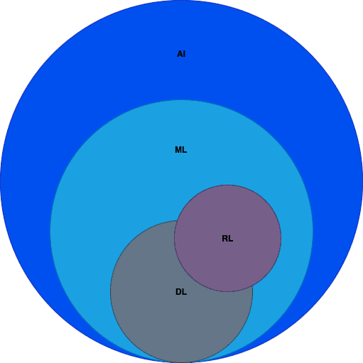
As for Reinforcement Learning, it is considered to be a Machine Learning problem as it does not require using DL techniques to solve it. However, there is a Deep Reinforcement Learning concept that is based on neural networks training. That is why Reinforcement Learning is somewhere in between ML and DL. Anyway, there is a clear borderline between DL and Reinforcement Learning concepts. In classical DL you use a neural network to learn on a training set and then use your model on a new data set. On the opposite, in Reinforcement Learning you learn dynamically by adjusting the agent’s actions based on continuous feedback.

How does Reinforcement Learning compare with other ML techniques?

Let’s make it clear once and for all. There are four classes of Machine Learning problems:

Supervised Learning – the data is labeled and you need to learn a function that maps an input to an output based on example input-output pairs
Unsupervised Learning – the data is not labeled and you need to find some structure in your data to formulate conclusions about it
Reinforcement Learning – you have an environment, an agent, a set of actions and you need to learn dynamically by adjusting the agent’s actions based on continuous feedback to maximize the overall reward
Semi-Supervised Learning – you need to solve some problem having a data set with both labeled and unlabeled data

As you might notice, there is a clear difference between all these classes, so it is really important to identify what Machine Learning problem you have to solve. To formulate an Reinforcement Learning problem you must fully understand the general Reinforcement Learning concept. Reinforcement Learning is about exploration as your agent tries different actions while finding a proper policy that will maximize the reward. That is the key difference between Reinforcement Learning and other types of learning. In other types of learning the concept is different. For example, in Supervised Learning agents learn simply by comparing their predictions with existing labels and updating their policies afterward.

How to formulate a basic Reinforcement Learning problem?

It might be tricky when identifying what ML problem class suits your task. However, it is crucial for the project’s success as you do not want to overcomplicate the task by using an irrelevant learning model and algorithm. Luckily it is quite easy to identify if Reinforcement Learning suits your problem and formulate a task.

All you need to do is just remember the Reinforcement Learning concept and understand if your task is an optimization problem. Also, you must explore the opportunities and figure out if there is any metric your Reinforcement Learning agent can maximize or minimize.

Reinforcement Learning step-by-step example

Let’s look at a simple example. Imagine you want to achieve a 100 score in Flappy Bird, but the game is quite challenging and you can not do it on your own, so you decide to use ML to solve this problem. To start with, you must identify the learning type that suits the problem.

The problem is an optimization task as you want to achieve a 100 score (you want to optimize your in-game actions in such a way that will give you a 100 score). The score itself seems like a nice metric to be optimized as it measures the player’s success in the game. Thus, it seems like Reinforcement Learning might be a good fit for this task.

Now, it is time to formulate the task. As you might remember when solving a Reinforcement Learning problem you need an agent, an environment, a set of actions, and some sort of reward policy. In this case, it is quite easy to identify all these components:

An agent is a bird itself
An environment is the Flappy Bird game
A set of actions has two possible actions: “click’ or “do not click”
You can come up with a reward policy yourself, but it seems reasonable to give your agent +1 if it is still alive and -1000 otherwise

As a state of the environment, you might use such parameters as:

If the agent is still alive
The horizontal distance from the next pair of pipes
The vertical distance to each pipe of the next pair
And many more (if you need them)

Image source: FlappyBirdRL

Thus, we have identified if RL suits the task and formulated an RL problem on a simple example.

Real-life applications of Reinforcement Learning

Now when you understand the basic concept of Reinforcement Learning let’s talk about some real-life applications. In general, Reinforcement Learning is used when there is the need to balance the delayed benefit with situational decision-making. So, Reinforcement Learning solves the difficult task of correlating the immediate actions with the delayed long-term reward they produce. Just like humans, Reinforcement Learning algorithms have to wait sometimes until they see the outcome of previous decisions.

Reinforcement Learning can be effectively applied in:

Planning – you will understand why a bit later
Bots for games – for example, AlphaGo Zero, Flappy Bird, Pacman e.t.c
Chat bots that learn from dialogue to dialogue
Trading bots
Robotics
Self-driving cars
Healthcare
And many more

How does Reinforcement Learning work?

Now you understand the basic concept of Reinforcement Learning. You also know how Reinforcement Learning is related to ML and DL, what the difference is between Reinforcement Learning and other types of learning, and where Reinforcement Learning can be applied. Moreover, you can formulate a Reinforcement Learning problem. Now let’s move on and discuss in-depth how Reinforcement Learning works.

The Bellman equation

Let’s start with some math and talk about the theoretical background of many Reinforcement Learning algorithms. As mentioned above Reinforcement Learning is based on the reward maximization hypothesis.

So, the best action an agent can perform is the one that maximizes the reward.

The reward at each time step t can be written as:

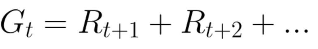
However, it is not that simple. You see, the rewards that an agent can get earlier are more likely simply because they are more predictable than future rewards. So, it will be better for us to decompose the reward function into the immediate reward and the discounted future rewards. That is where the Bellman equation comes in.

Bellman expectation equation

In general form, the Bellman equation looks as follows:

The equation states the reward for acting a in state s must be divided into two parts. The first one is the immediate reward r which an agent will get for acting a. The second one is a discounted reward for the best action in the next state (when the action a in state s is performed the agent transitions to a new state). The discount value 𝞬 indicates that receiving the reward right now is more valuable rather than receiving the reward in the future. That is why 𝞬 which is a number between 0 and 1 (usually 0.9 to 0.99) is multiplied by the reward in the future devaluing the future rewards.

So, why do you need to penalize future rewards? Well, it seems logical as these rewards have higher uncertainty. You do not know if you get it at all. Moreover, having an immediate reward is more likable than hoping to have something in the future.

As you might notice, the Bellman equation is recursive, so it describes a whole Reinforcement Learning process step-by-step.

Bellman's principle of optimality

The Bellman expectation equation is based on Bellman’s principle of optimality. The principle states that “an optimal policy has the property that whatever the initial state and initial decision is, the remaining decisions must constitute an optimal policy with regard to the state resulting from the first decision”. In other words, the optimal strategy depends only on the current state and overall goal and does not depend on the background.

Thus, if you have complete information about the environment a Reinforcement Learning problem turns into a planning problem and does not require using advanced ML techniques at all. Unfortunately, in real life, it is a rare case. That is why there are many Reinforcement Learning algorithms including neural networks.

Markov Decision Process

The majority of Reinforcement Learning problems can be formed as a Markov Decision Process (MDP). A Markov Decision Process is a representation of the sequence of actions of an agent in an environment and their consequences on not only the immediate rewards but also future states and rewards. All states in MDP must satisfy the Markov Property which states that the new state depends only on the preceding state and action and is independent of all previous states and actions. As you might notice, MDP nicely correlates with the Bellman expectation equation.

Below there is an example of a simple MDP. In this case, an MDP has three states marked with green circles (S0, S1, S2) and two actions (a0, a1) marked with orange circles that an agent can perform to transition from one state to the other. The orange arrows are the rewards an agent gets if it performs a certain action. Numbers beside the black arrows are transition probabilities. These are probabilities of transitioning from one state to another after the act. For example, if you are currently in state S1 and act with a0 there is a 70% probability that you will transition to state S0.

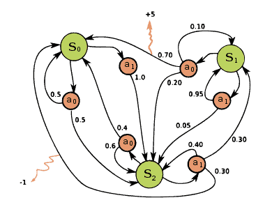
Image source: Wikipedia

So, we can easily define an MDP using a set of possible states and actions, transition probabilities, a reward function, and discount value 𝞬 that will be used to devalue future rewards.

Key Concepts of Reinforcement Learning

Now when you know some theoretical background, let’s take a step back and discuss the Reinforcement Learning concept from another perspective.

Model of an environment

As you might already figure out an MDP is a model that describes the Reinforcement Learning environment. It states how an environment will react to certain actions by defining transition probabilities and reward function. Therefore, there are two different scenarios, either you know the model or you do not.

As mentioned above, if you know the model (you have the complete information about the environment including transition probabilities and reward function) you will face a model-based Reinforcement Learning problem that is pretty similar to planning. Such a problem can be easily solved using Dynamic Programming. Unfortunately, in most cases, you will not know the model. Thus, you face a model-free Reinforcement Learning problem or try to figure out the initial model while training. Anyway, that is when Machine and Deep Learning techniques come in handy.

One way or another in Reinforcement Learning you will try to learn two things: agent’s policy and value functions.

Agent’s Policy and Value functions

Agent’s policy is a guideline that advises which action to perform in a given state to try and maximize the overall reward. As for value functions, these are functions that predict the future rewards for acting a certain way in a given state.

In other words, a value function shows if a state or an action is rewarding and worth taking. The future rewards are predicted using the Bellman expectation equation. Using value functions you can calculate such values as:

State-value – your expected reward if you are in state S at given time T
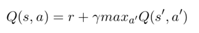
Action-value (it is usually referred to as Q-value and is written as Q (s, a)) – your expected reward if you act A being in state S at given time T

Moreover, you can subtract the action-value from the state-value and find out the advantage you might get if you act instead of doing nothing.

It all comes together when thinking about optimal policy. Let’s make this clear. Your agent wants to find the most optimal value functions as it wants to get the maximum return. Thus, it will be able to formulate the policy as it consists of the optimal value functions.

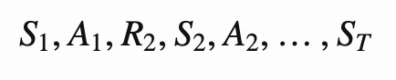
SARS-chain

It is worth mentioning that the Reinforcement Learning process is usually formalized using a SARS-chain. The learning process can be easily divided into blocks called episodes that contain the state, action, and reward for this action. In the picture below you can find such a chain. In this picture the state is St, the action is At, and the reward is Rt

How to solve a Reinforcement Learning problem?

To start with let’s define some useful terms that are commonly used when describing a Reinforcement Learning algorithm

Reinforcement Learning algorithms

Model-free algorithms are the ones that do not use the environment’s model while training

Model-based algorithms are the ones that are based on the environment’s model. Still, it means that you must either know the model or figure it out while training

Value-based algorithms are the ones that maximize a value function. An agent in these algorithms is expecting long-term rewards of the current states under specific policy

Policy-based algorithms are the ones that try to learn such a policy that each action taken in every state will lead to the maximum possible reward in the future

On-Policy vs. Off-Policy

It is important to understand how On- and Off-Policy algorithms are actually different. From the general perspective, it might seem that in the on-policy case an agent simply follows options whereas in the off-policy case he explores. However, it is not what separates on-policy from off-policy algorithms.

Let’s define two additional terms that will help us see the difference. These are update policy and behavior policy. Update policy is how your agent learns the optimal policy. Behavior policy is how your agent behaves in a given situation.

In on-policy algorithms, the agent uses a single policy both as the update and behavior policy. On the other hand, in off-policy algorithms, update and behavior policies are different. You will see a clear difference in examples later on when we cover the algorithms themselves.

Types of Reinforcement Learning

Also, there are two types of Reinforcement Learning methods you need to know:

Positive RL
Negative RL

The difference is clear and easy to understand. In Positive Reinforcement Learning you need to add something to increase the likelihood of certain behavior. There are many examples of Positive Reinforcement Learning in our everyday life as it is the most effective way to teach a person or an animal to do something new. Let’s return to the dog training example. When your dog performs as intended you give it a treat. From the Reinforcement Learning perspective, you give it positive stimuli. Thus, you increase the likelihood of the dog behaving the necessary way in a similar situation.

In Negative Reinforcement Learning you need to remove something to increase the likelihood of a behavior. Negative Reinforcement Learning is less used, still, there are examples from everyday life. For example, you face Negative Reinforcement Learning if you do not fasten your seatbelt when driving a car. In such a case, your car will make a loud and annoying noise until you buckle up for safety. Thus, you will stop the noise by acting the intended way. This increases the likelihood of similar behavior next time.

Dynamic Programming

Dynamic Programming is a broad mathematical optimization and computer programming sphere. As mentioned above when you face a model-based Reinforcement Learning problem you can successfully solve it by using it. This is possible because you have the complete model of your environment. Therefore, Dynamic Programming algorithms following Bellman’s equations can easily find an optimal policy for your agent to follow.

The general idea of Dynamic Programming is to divide a problem into subproblems, solve them, and store the results for the further optimal solution exploration. To solve a Dynamic Programming problem you need to somehow evaluate policies and find an optimal one for the given problem. There are three concepts designed to help you with that:

Policy Evaluation
Policy Improvement
Policy Iteration

Policy Evaluation is a technique that helps to identify how good a current policy is. In the first iteration, for example, your agent’s policy might be random acting. Policy Evaluation is based on iteratively calculating state-value functions until it converges to the true value function of a given policy (until the maximum state-value functions maximum change is less than some user-specified constant). If you want to check a general algorithm please refer to the video explanation on Coursera.

Now, when you know how to evaluate a policy using the value function it is time to improve it and find better policies. Imagine you have determined the value function for your initial policy. As you want to make some improvements you start exploring and wonder what will happen if for some state S you choose an action A that does not correspond to your initial policy. Let’s make this clear. You know the current policy from S, but you want to find out if it would be better or worse to change to the new policy. Therefore, you choose A in S and then follow the initial policy. Thus, you will be able to compare two values: the one from the initial value function I and the one from the updated U.

If I is greater than U, then you can expect it will be better to select A every time you occur in S. That will formulate a new policy that will presumably be a better one. All mentioned above was a special case of the Policy Improvement theorem.

However, to guarantee the result you need to follow the Generalized Policy Iteration (GPI) algorithm. GPI combines Policy Evaluation and Policy Improvement in an iterative cycle that will ensure the improvement given enough iterations. However, the GPI algorithm is iterative which means it is time-consuming.

In the picture below you can see the workflow of GPI. E stands for Policy Evaluation, I for Policy Improvement, π for policy, and v for value function.

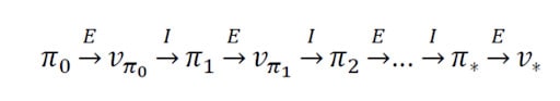
Image source: Dynamic Programming

Episodic Vs. Continuous task

A task is an instance of a Reinforcement Learning problem. There are two types of tasks:

Episodic
Continuous

In the episodic task case, you have a start point and an end point (terminal state). This defines an episode: a list of states, actions, rewards, and new states between the start point and the terminal state. For example, in Super Mario Bros the episode starts with the launch of a new Mario and ends when you are killed or reach the end of the level.

Image source: Super Mario Bros.

Continuous tasks are the tasks that can go on forever as they do not have the terminal state. In such a task, the agent must learn to choose the best actions and simultaneously interact with the environment. For example, an agent who performs automated stock trading. There is no starting point or terminal state for this task. The agent continues to work until you decide to stop him.

Monte-Carlo method

Monte-Carlo is a model-free method that learns from episodes of experience. When an episode ends (the agent reaches the terminal state), it looks at the total accumulated reward to evaluate how well it did. In the Monte-Carlo approach, the reward is obtained only at the end of the game. Then it starts an episode from the very beginning with the augmented knowledge it gained from the previous approach. The agent improves its decisions with each iteration.

From the mathematical point of view, the Monte-Carlo method can be described with the following formula:

In this formula:

V (St) on the left stands for the maximum expected future reward starting at state St
Other V (St) in the formula are the former estimation of maximum expected future reward starting at state St
α is a learning rate
Gt is discounted cumulative reward

Let’s look at an example.

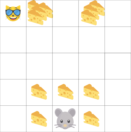
Imagine that the labyrinth is your environment and the mouse is your agent:

You will always start from the same start point (the middle of the bottom line)
You will reach the terminal state and end the episode if the cat eats the mouse or, for example, if the agent moves on more than 20 steps. You need that additional terminal state to end the episode even if your agent survives
At the end of the episode, you will get a list of states, actions, rewards, and new states that occurred during the episode
The agent sums up the total reward to check how well he did
Then it updates V (St) according to the above formula.
Then the episode will launch from the beginning but with new knowledge. As you might notice, the idea is pretty similar to GPI

Thus, by launching more and more episodes, the agent will learn to play even better.

Temporal-Difference Learning

Temporal Difference (TD) Learning is similar to the Monte-Carlo method. However, despite it learning from episodes of experience and being model-free, TD has a unique feature. TD will not wait for the episode to end to update the maximum possible reward. The reward will be updated during the episode based on gained experience.

This method is called TD (0) or incremental TD (updates the value function after every single step). Let’s compare the TD Learning formula with the Monte-Carlo formula:

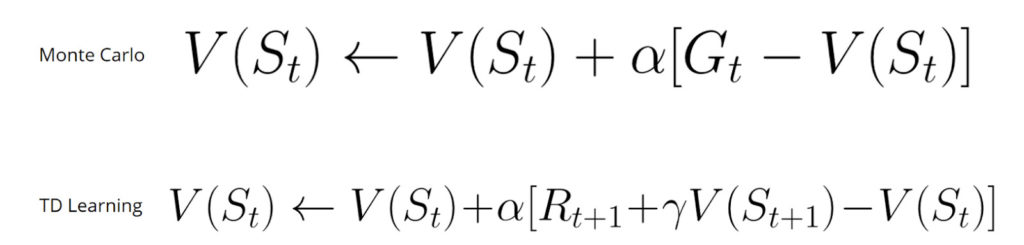
In the TD formula:

V (St) on the left stands for the maximum expected future reward starting at state St
Other V (St) in the formula are the former estimation of maximum expected future reward starting at state St
α is a learning rate
Rt + 1 is the expected
reward on time step t + 1
γV (St + 1) is the discounted value on the next step
Rt + 1 + γV (St + 1) part of the formula is called a TD target

TD methods update values each time step. At time step t + 1, a TD target is generated using the reward Rt + 1 and the current estimate V (St + 1). The ultimate goal of TD is to estimate the expected values. This is the key difference between Temporal-Difference Learning and Monte-Carlo method. TD works with existing estimates whereas the Monte-Carlo method relies on immediate and complete rewards. The TD approach is called bootstrapping.

Now, when you understand the concept of Temporal-Difference Learning it is time to figure out how to learn an optimal policy in TD. There are two basic approaches that will be shown on two famous Reinforcement Learning algorithms:

SARSA
Q-Learning

SARSA

SARSA is the on-policy TD control algorithm. It can be visualized using SARS-chains and is pretty similar to the GPI when learning an optimal policy.

The general SARSA algorithm is as follows:

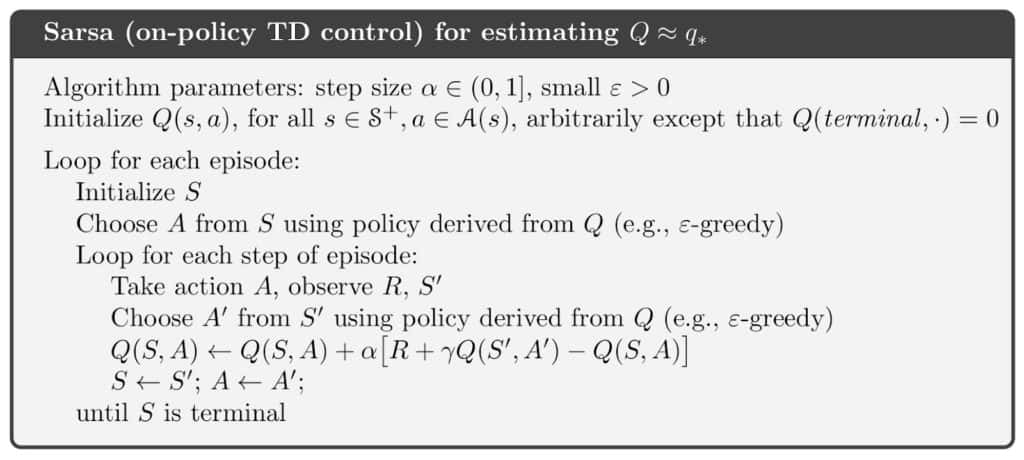
Image source: SARSA

Q-Learning

Q-Learning is the off-policy TD control algorithm. The general Q-Learning algorithm is as follows

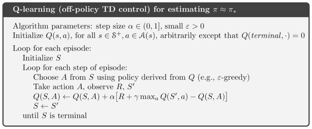
Image source: Q-Learning

SARSA Vs. Q-Learning

As you might notice in the pictures above both SARSA and Q-Learning are pretty similar. Still, there is one major difference. It all comes down to the On- and Off-Policy natures of the algorithms.

As mentioned above, Q-Learning is the Off-Policy algorithm. Thus, it learns the optimal policy using absolutely greedy policy and behaves using other policies, for example, ε-greedy policy to balance exploration and exploitation. In other words, the Q-Learning algorithm estimates the total discounted future reward for state-action pairs assuming a greedy policy was followed despite the fact that it is not following a greedy policy. On the other hand, SARSA being a typical example of On-Policy algorithm learns optimal policy and behaves using the same policy. Usually, it is ε-greedy policy.

How to implement Q-Learning in Python?

I have prepared a Google Collab notebook for you featuring working with Q-Learning using OOP techniques. In this notebook, we will try to solve a mini-game Reinforcement Learning problem on the n x n field. Rules are simple, the agent must hold out as long as possible at a distance from the opponents that move at random. The task of the opponents is to catch the agent. The agent is rewarded for each turn it survives. Please feel free to experiment and play around as there is no better way to master something than practice.

Deep Q-Network

The Deep Q-Network (DQN) algorithm developed in 2015 is a logical improvement of the existing approaches. It was able to solve a wide range of Atari games by combining Reinforcement Learning and deep neural networks at scale. The algorithm enhances Q-Learning with deep neural networks and the experience replay technique. The general algorithm of the DQN is as follows:

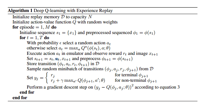
In DQN, the current state is given as the input to the neural network. The output of the neural network is the number Q (s, a) for all possible actions. Thus, it turns out that the neural network in DQN implements the classical function Q (s, a) from Q-Learning. You simply get the usual argmax over the network outputs array and choose the action with the highest Q (s, a). Unfortunately, DQN works only with discrete actions. Continuous case is the bottleneck of this approach.

As mentioned above the DQN benefits from using the experience replay technique. Experience replay requires storing all the episode steps that can be visualized in the SARS-chain (St, At, Rt, St + 1) form in one replay memory. During Q-Learning updates a random batch of samples is drawn from the memory and the update is made based on this mini-batch. Samples from the batch are then returned to the replay memory. Such an approach removes correlation in the observation sequences and gives Q-Learning a nice boost.

Policy Gradient

Let’s change the logic a bit. The current state will be the input, but as the output, the network will predict the actions themselves or the probability distribution for them. The agent will follow the neural network prediction and act as suggested. When the episode ends you will be able to calculate the cumulative reward the agent got for the episode.

The key idea is to use the dynamics of the received reward to calculate the gradient using the Policy Gradient Theorem, apply it to the weights of the neural network, and use the simple backpropagation. The idea is simple yet powerful. You can not use actions as the output labels to compute the gradient as you simply do not know what they should be. Still, you can use the reward change to calculate the gradient. The network will learn from this gradient to predict the actions that lead to an increase in the reward.

This approach is known as the Policy Gradient algorithm. However, a major drawback is that you have to wait till the end of the episode to calculate the cumulative reward before changing the network weights according to it.

There are many variations of the Policy Gradient algorithm. However, one of the most classic Policy Gradient algorithms is REINFORCE.

The REINFORCE algorithm is as follows:

Initialize a policy (even random)
Give the current state to the neural network as the input and receive the probability distribution for them
Play some steps of the environment and record the actions your agent performed
Calculate the discounted reward for each played via backpropagation
Calculate the expected reward
Adjust weights of the initial policy using backpropagation error in the neural network. Thus, you will increase the expected reward
Repeat from step 2 until your agent is trained

Actor-Critic

Now imagine that we have two networks: one predicts what actions should be performed, and the second assesses how good these actions are in the grand scheme of things. To make things clear, the second network outputs the Q-value for these actions as in the DQN algorithm.

The first network is usually referred to as an Actor and has a current state as an input, and action as the output. The input for the second network known as Critic is both a current state and an action predicted by the first network. As the output, it predicts the Q (s, a).

The Critic’s output Q (s, a) can be used to calculate the gradient. Then the gradient is used to update the Actor’s weights. This approach is called Actor-Critic. A clear advantage over the classic Policy Gradient is that the network weights can be updated at every step, without waiting for the end of the episode. Thus, Actor-Critic trains a bit faster.

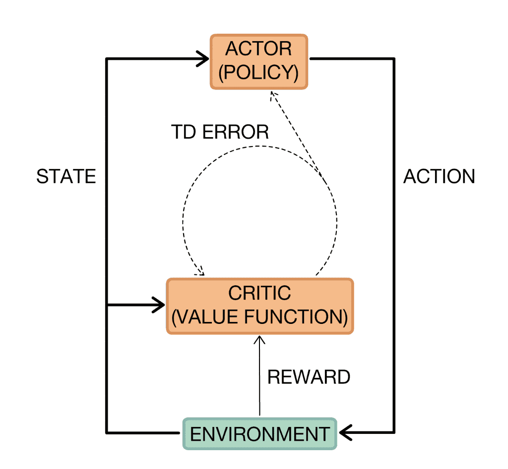
Image source: Actor-Critic

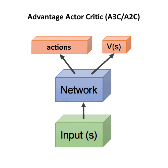
Asynchronous Advantage Actor-Critic

Asynchronous Advantage Actor-Critic known as A3C is the next iteration of the classic Actor-Critic algorithm. It is based on the biological concept stating that the maximum release of dopamine occurs not during the pleasure itself, but the expectation of the future pleasure. In A3C a gradient is calculated using a value that shows how much better or worse the actions predicted by Actor were than we expected.

So, in A3C there is a new value called Advantage used to calculate the gradients: A (s, a) = Q (s, a) – V (s). The A (s, a) value shows if it would be better in the grand scheme of things to perform an action a in the current situation V (s). If A (s, a) > 0, then the gradient will change the weights of the neural network, encouraging the actions predicted by the network. If A (s, a) < 0, the gradient will change the weights in the opposite direction. The predicted actions will be suppressed since they turned out to be bad.

In this Advantage formula, V (s) shows how good the current state is on its own, without being bound to actions (therefore, it only depends on s, without a). If we are one step away from the summit of Everest, this is a very good state situation, with a large V (s). And if we have already fallen out and are falling, then it is obviously a bad state with a low V (s). Fortunately, with this approach, Q (s, a) can be replaced with the reward r, which an agent gets after the action. Thus, the Advantage formula will be A = r – V (s).

In this case, you need to predict only V (s) and both actor and critic can be combined into one neural network that will receive the current state as an input, and split into two heads at the output: one will predict actions, and the other will predict V (s). However, you can use two separate networks as well.

Challenges of Reinforcement Learning

Reinforcement Learning comes with multiple challenges and dilemmas. In general, they can be divided into two big group

Obstacles that may occur when working on an Reinforcement Learning project
Global Reinforcement Learning challenges

For example, in the first group there such obstacles as:

Incredibly long training time
Non-stationary, complicated or partially observable environments
Irrelevant reward function
Irrelevant algorithm or outdated library
And many more

Still, Reinforcement Learning has global challenges, for example, the exploration-exploitation problem or the Deadly Triad issue.

The exploration-exploitation trade-off is a well-known dilemma for Reinforcement Learning algorithms. Unfortunately, this problem occurs when a learning algorithm has to make a lot of decisions with an uncertain pay-off. In general, the dilemma states as follows. A learning algorithm that has incomplete knowledge of the world can either perform the same actions that have been successful so far to maximize the overall reward or it can try something new hoping to get an even greater reward. So, the algorithm either exploits or explores, but a good algorithm needs to find a balance between these two approaches which can be a non-trivial task.

The Deadly Triad problem refers to the situation when bootstrapping, Off-Policy, and nonlinear function approximations are combined in one Reinforcement Learning algorithm. In such a case, training might be unstable and hard to converge. However, as of today, many Deep Reinforcement Learning architectures avoid this problem. Still, you need to be careful as the Deadly Triad problem is more than real.

Reinforcement Learning vs. Supervised Learning

As you might remember, we have already compared Reinforcement Learning with other ML learning methods at the beginning of the article. Still, to make things clear let’s compare Reinforcement and Supervised Learning (SL) one more time. The difference between them is not that obvious as both Reinforcement Learning and SL are considered to be the learning method with the teacher.

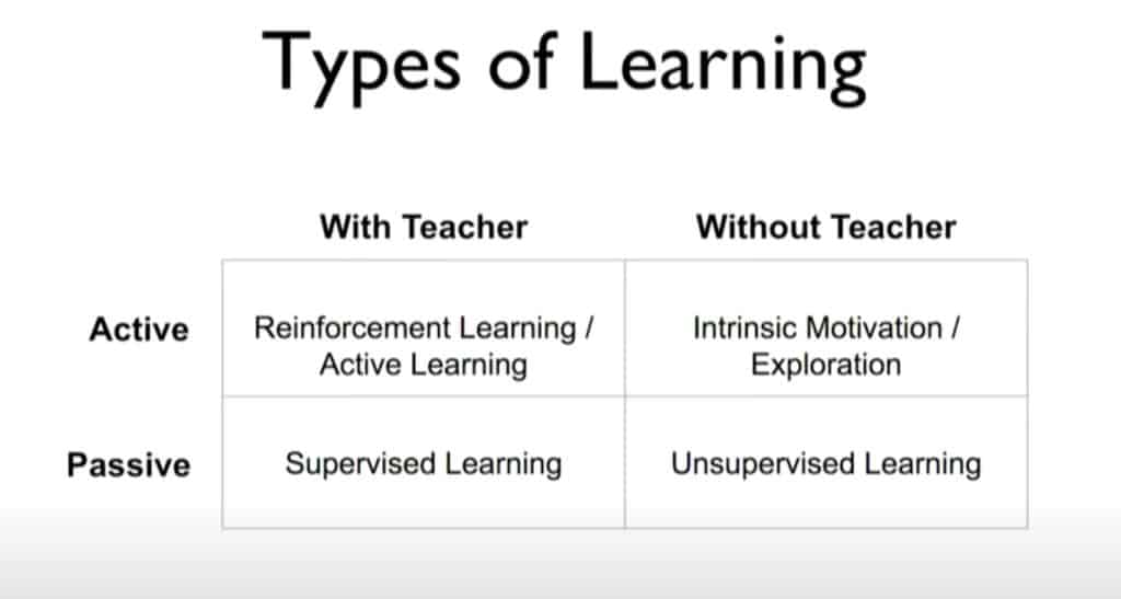
Image source: YouTube

Supervised Learning has the passive learning process with the instructive role of the teacher. The passive learning process means that a model simply maps input space to output space. It does not change the input space as a result of learning. The instructive role of the teacher means that the teacher gives a model some feedback about its performance. For example, in the case of a Classification problem, the feedback might be the probabilities of an object belonging to classification classes. The model uses this feedback to adjust its performance during training.

On the other hand, Reinforcement Learning has the active learning process with the evaluative role of the teacher. The active learning process means that the agent learns by interacting with the environment around it (the environment is the input space). Thus, it changes the environment thereby constantly changing the input space. The evaluative role of the teacher means that an Reinforcement Learning agent does not receive feedback for every action it performs. Instead, the overall feedback is some cumulative average measure of some metric that is the consequence of the effect of all the actions the agent made.

Why should you try Reinforcement Learning?

There is an opinion that Reinforcement Learning is overhyped and is not that useful in the industry. On the opposite, some specialists believe that Reinforcement Learning is the future. Anyway, there are reasons for you to try Reinforcement Learning:

It is a commonly used learning method in everyday life. Nowadays, thanks to advanced technologies Data Scientists can unveil its true potential and apply Reinforcement Learning in multiple spheres
Some tasks simply cannot be solved without RL
It provides many insights as it shows which action leads to the highest long-term reward
It provides you with the optimal policy for a given environment
It provides you with a trained agent that can be used for similar tasks

When to use and not to use Reinforcement Learning?

This question might be a little tricky, however, there are valuable tips that will help you decide if you should try Reinforcement Learning or not.

You should try using Reinforcement Learning if:

Reinforcement Learning fits your problem
You can describe the environment using quantitative variables. Moreover, you must be able to access these variables at each time step or state
You have a reward function that you can maximize or minimize
You have time for research, exploring the opportunities, and waiting while your agent trains

You should not use Reinforcement Learning if:

Reinforcement Learning does not fit your problem
You have enough data to solve your problem using another learning technique, for example, Supervised Learning
You do not have enough time both for research and training

How to get started with studying Reinforcement Learning?

Reinforcement learning is a field that you need to study before you start using it effectively. Unfortunately, it requires knowledge in many spheres including mathematics and statistics, Machine and Deep Learning. Thus, you should definitely check some reliable and valuable tutorials, courses, and projects to get things going.

There are some things I can recommend you:

Fundamentals of Reinforcement Learning course on Coursera
Reinforcement Learning course on Coursera
Introducing to Reinforcement Learning in Python course on Coursera
Practical Reinforcement Learning course on Coursera
Flappy Bird tutorial
Introduction to Reinforcement Learning article
Mario tutorial and Mario project
Check Kaggle. There might be something interesting
Simply Google your task. It is likely you will find something similar

Final Thoughts

Hopefully, this tutorial will help you succeed and use Reinforcement Learning whenever you need it.

To summarize, we started with the general Reinforcement Learning concept and the technique to formulate an Reinforcement Learning problem. Then, we have covered some mathematical background behind Reinforcement Learning. Also, we talked about many Reinforcement Learning algorithms and covered the Python implementation of Q-Learning. Lastly, we mentioned challenges, use cases, and valuable tutorials, courses, and projects.

If you enjoyed this post, a great next step would be to start studying Reinforcement Learning by yourself with all the relevant tools mentioned in this article.

Thanks for reading, and happy training!

Resources

Top MLOps guides and news in your inbox every month