Table of Contents
What is Image Segmentation?
Image segmentation is the art of partitioning an image into multiple smaller segments or groups of pixels, such that each pixel in the digital image has a specific label assigned to it. Pixels with the same label have similarity in characteristics.
After segmentation, the output is a region or a structure that collectively covers the entire image. These regions have similar characteristics including colors, texture, or intensity.
Modes and types of segmentation
Image segmentation is divided into two groups, which include:
- Semantic segmentation – This refers to the process of detecting class labels for every pixel. For example, in a picture with cars and people, cars will be segmented as one object and people as another object.
- Instance Segmentation – This refers to the process of detecting an instance of an object for every pixel. For example, in a picture with cars and people, each car will be detected as an individual object as well as every person.
In computer vision, this is useful because it can be applied in several areas including controlling traffic by counting the number of cars.
Why do we Need Image Segmentation?
Image segmentation is important because it can enhance analysis of images with more granularity. It extracts the objects of interest, for further processing such as description or recognition. Unlike other types of image processing techniques, Image segmentation can detect the edges, boundaries and outlines within an image. It’s used in various applications and has helped to build some life-changing and even life-saving technologies across industries.
Image Segmentation is already being applied in a number of fields which include:
- Medical Imaging including CT and MRI, cancer cell detection etc
- Machine vision used in self-driving vehicles and robotics
- Face recognition and detection
- Video surveillance systems
- Satellite imaging among others
Image segmentation techniques
We can use different types of techniques to partition images into different segments. This section will cover 3 common techniques.
- Region-based segmentation
- Edge detection segmentation
- Clustering methods
Region-based Segmentation
The region-based segmentation technique looks for similarities between two adjacent pixels, then similar pixels are grouped into a similar region while the unique ones are grouped into different regions. There are a number of approaches to achieve this, and in this example, we are going to implement a threshold-based approach.
First, let’s import all the necessary libraries
					from skimage.color import rgb2gray
import numpy as np
import cv2
import matplotlib.pyplot as plt
%matplotlib inline
from scipy import ndimage
Read image and convert to grayscale
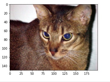
					image = plt.imread('images/cat.jpg')
image.shape
plt.imshow(image)
					gray = rgb2gray(image)
plt.imshow(gray, cmap='gray')
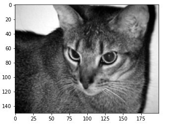
Check image shape
gray.shape
(150, 200)
Finally, let’s take the mean of the pixels as our threshold value, and any value above the mean we set it as the background and value below the threshold, we set it as the object.
					gray_r = gray.reshape(gray.shape[0]*gray.shape[1])
for i in range(gray_r.shape[0]):
    if gray_r[i] > gray_r.mean():
        gray_r[i] = 1
    else:
        gray_r[i] = 0
gray = gray_r.reshape(gray.shape[0],gray.shape[1])
plt.imshow(gray, cmap='gray')
Output
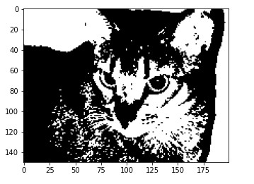
For better results, you can adjust your threshold value. Also, you can create multiple segments by changing the logic of the threshold.
Advantages Region-based Segmentation
- Easy to implement
- Faster calculation speed.
- Performs well when the object and background have higher contrast.
Limitations of Region-based Segmentation
- Performs poorly when the contrast between the object and background is lower.
Edge detection segmentation
Edges separate different regions in an image since there is usually a sharp adjustment in intensity at the region boundary. We can take advantage of these sharp adjustments to detect the boundaries of objects using filters and convolutions.
Types of Edge detection operators
- Gradient-based operator computes first order derivations in an image, examples of these operators include Sobel operator, Robert operator, and Prewitt operator.
- Gaussian based operator computes second-order derivations in an image, examples of these operators include Canny edge detector and Laplacian of Gaussian
Below is a step-by-step example of using python to implement edge detection segmentation. In this example, we shall be implementing a Sobel operator.
Sobel operators use two weight matrices, one for detecting horizontal and another one for detecting vertical edges.
Horizontal Sobel
1 | 2 | 1 |
0 | 0 | 0 |
-1 | -2 | -1 |
Vertical Sobel
-1 | 0 | 1 |
-2 | 0 | 2 |
-1 | 0 | 1 |
This is going to work by convolving these filters over an image
First, let’s import all the necessary libraries, load an image and visualize
import numpy as np
import matplotlib.pyplot as plt
%matplotlib inline
from scipy import ndimage
from skimage.color import rgb2gray
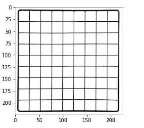
image = plt.imread('images/edge image.png')
plt.imshow(image)
Next, let’s convert the image to grayscale and define our Sobel operator
					gray = rgb2gray(image)

sobel_horizontal = np.array([np.array([1, 2, 1]), np.array([0, 0, 0]), np.array([-1, -2, -1])])
sobel_vertical = np.array([np.array([-1, 0, 1]), np.array([-2, 0, 2]), np.array([-1, 0, 1])])
Next, let’s convolve the filter over the image
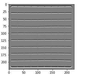
out_h = ndimage.convolve(gray, sobel_horizontal, mode='reflect')
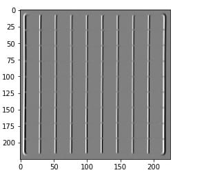
out_v = ndimage.convolve(gray, sobel_vertical, mode='reflect')
Display horizontal edges
plt.imshow(out_h, cmap='gray')
Display vertical edges
plt.imshow(out_h, cmap='gray')
Advantages of edge detection segmentation
- Simple to implement
- Easy when searching for smooth edges
Limitations of edge detection segmentation
- Highly sensitive to noise
- Limited accuracy
Clustering-based segmentation
K-Means clustering is a clustering Algorithm that splits data into k different clusters. We can as well use this algorithm in image segmentation to generate object segments. Below is an example based on K-Means and Opencv.
First, import the necessary libraries
					import numpy as np
import cv2
import matplotlib.pyplot as plt
Load image and show using `matplotlib` `imshow()` method
					original_image = cv2.imread('images/environment.jpeg')
plt.imshow(original_image)
Convert your image from RGB Colours Space to HSV
					img = cv2.cvtColor(original_image, cv2.COLOR_BGR2RGB)
plt.imshow(img)
When clustering the image using k-means, we first need to convert it into a 2-dimensional array whose shape will be (length*width, 3) and convert it to unit 8 value using float 32 as required by OpenCV.
					vectorized = img.reshape((-1,3))
vectorized = np.float32(vectorized)
Next, let’s define k, attempts, and criteria as required by K-Means as a parameter
					criteria = (cv2.TERM_CRITERIA_EPS + cv2.TERM_CRITERIA_MAX_ITER, 10, 1.0)
K = 3
attempts=10
ret,label,center=cv2.kmeans(vectorized,K,None,criteria,attempts,cv2.KMEANS_PP_CENTERS)
Next, let’s convert back to uint8, and let’s get the clustered image.
					center = np.uint8(center)

res = center[label.flatten()]
result_image = res.reshape((img.shape))
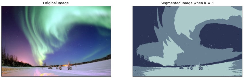
Finally, display the clustered image
					figure_size = 15
plt.figure(figsize=(figure_size,figure_size))
plt.subplot(1,2,1),plt.imshow(img)
plt.title('Original Image'), plt.xticks([]), plt.yticks([])
plt.subplot(1,2,2),plt.imshow(result_image)
plt.title('Segmented Image when K = %i' % K), plt.xticks([]), plt.yticks([])
plt.show()
Advantages of Clustering-based Segmentation technique
- Generate excellent clusters in small datasets
Limitations of Clustering-based Segmentation technique
- Computation time is too long for a larger dataset
- Not suitable for clustering non-convex clusters
Summary of Image segmentation techniques
Technique | Description | Pros | Cons |
Region-based segmentation | Region-based segmentation technique looks for similarities between two adjacent pixels, then similar pixels are grouped into a similar region |
|
|
Edge detection segmentation | Takes advantage of these sharp adjustments to detect boundaries of objects using filters and convolutions. |
|
|
Clustering methods (K-Means) | Splits an image into k different splits |
|
|
How Image Segmentation Works
Image segmentation works by using encoders and decoders. Encoders take in input, which is a raw image, it then extracts features, and finally, decoders generate an output which is an image with segments.
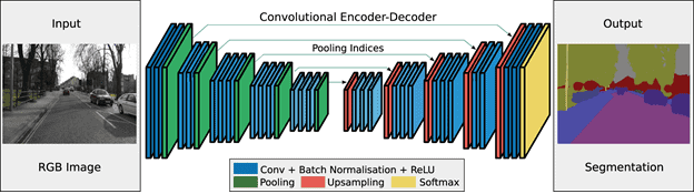
The basic model of an image segmentation
Image segmentation architectures
In deep neural networks, architecture defines the involvement of each layer in the machine learning cycle. Since each model is built to handle different activities, it is common for them to have different structures. In image segmentation, we are going to discuss the most common architectures which include U-Net, FastFCN, Deeplab, Mask R-CNN, etc.
U-Net
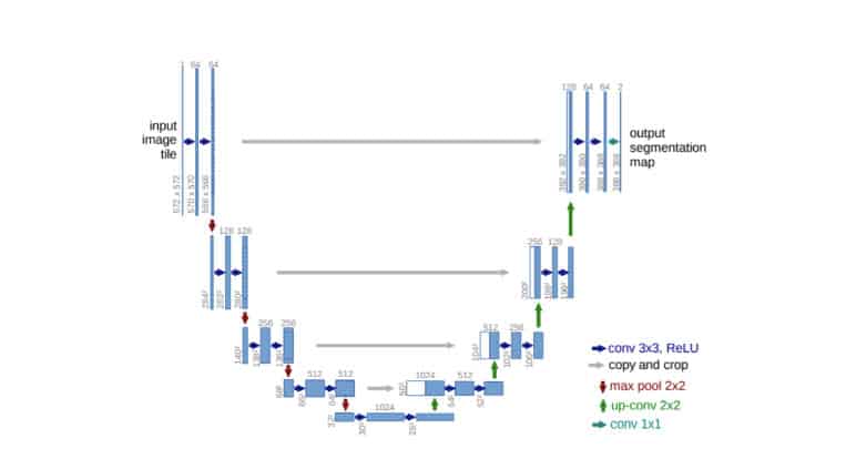
U-Net architecture is a deep learning image segmentation architecture introduced by Olaf Ronneberger, Philipp Fischer and Thomas Brox in 2015. It’s an encoder-decoder architecture convolutional neural network that was specifically designed to be used in Biomedical Imaging.
The main goal for this architecture was to tackle two important issues in the field of medical imaging which are:
- Lack of large training datasets – Traditional convolutional neural networks with fully connected layers, require large datasets because of the large number of parameters needed to learn. Since medical imaging has small datasets, this architecture ensures maximum learning from the information provided because a fully connected layer is replaced with series of up convolutions on the decoder side.
- Capturing context accurately at different resolutions and scales.
Its U shape design consists of two parts. The left side is known as the contracting path or encoder path, where repeated typical convolutions are applied followed by ReLU and max pooling operations. The right side is known as the expansive path which has transposed 2D convolutional layers where upsampling technique is performed.
Implementation of UNet
					def build_model(input_layer, start_neurons):
    conv1 = Conv2D(start_neurons * 1, (3, 3), activation="relu", padding="same")(
        input_layer
    )
    conv1 = Conv2D(start_neurons * 1, (3, 3), activation="relu", padding="same")(conv1)
    pool1 = MaxPooling2D((2, 2))(conv1)
    pool1 = Dropout(0.25)(pool1)

    conv2 = Conv2D(start_neurons * 2, (3, 3), activation="relu", padding="same")(pool1)
    conv2 = Conv2D(start_neurons * 2, (3, 3), activation="relu", padding="same")(conv2)
    pool2 = MaxPooling2D((2, 2))(conv2)
    pool2 = Dropout(0.5)(pool2)

    conv3 = Conv2D(start_neurons * 4, (3, 3), activation="relu", padding="same")(pool2)
    conv3 = Conv2D(start_neurons * 4, (3, 3), activation="relu", padding="same")(conv3)
    pool3 = MaxPooling2D((2, 2))(conv3)
    pool3 = Dropout(0.5)(pool3)

    conv4 = Conv2D(start_neurons * 8, (3, 3), activation="relu", padding="same")(pool3)
    conv4 = Conv2D(start_neurons * 8, (3, 3), activation="relu", padding="same")(conv4)
    pool4 = MaxPooling2D((2, 2))(conv4)
    pool4 = Dropout(0.5)(pool4)

    # Middle
    convm = Conv2D(start_neurons * 16, (3, 3), activation="relu", padding="same")(pool4)
    convm = Conv2D(start_neurons * 16, (3, 3), activation="relu", padding="same")(convm)

    deconv4 = Conv2DTranspose(
        start_neurons * 8, (3, 3), strides=(2, 2), padding="same"
    )(convm)
    uconv4 = concatenate([deconv4, conv4])
    uconv4 = Dropout(0.5)(uconv4)
    uconv4 = Conv2D(start_neurons * 8, (3, 3), activation="relu", padding="same")(
        uconv4
    )
    uconv4 = Conv2D(start_neurons * 8, (3, 3), activation="relu", padding="same")(
        uconv4
    )

    deconv3 = Conv2DTranspose(
        start_neurons * 4, (3, 3), strides=(2, 2), padding="same"
    )(uconv4)
    uconv3 = concatenate([deconv3, conv3])
    uconv3 = Dropout(0.5)(uconv3)
    uconv3 = Conv2D(start_neurons * 4, (3, 3), activation="relu", padding="same")(
        uconv3
    )
    uconv3 = Conv2D(start_neurons * 4, (3, 3), activation="relu", padding="same")(
        uconv3
    )

    deconv2 = Conv2DTranspose(
        start_neurons * 2, (3, 3), strides=(2, 2), padding="same"
    )(uconv3)
    uconv2 = concatenate([deconv2, conv2])
    uconv2 = Dropout(0.5)(uconv2)
    uconv2 = Conv2D(start_neurons * 2, (3, 3), activation="relu", padding="same")(
        uconv2
    )
    uconv2 = Conv2D(start_neurons * 2, (3, 3), activation="relu", padding="same")(
        uconv2
    )

    deconv1 = Conv2DTranspose(
        start_neurons * 1, (3, 3), strides=(2, 2), padding="same"
    )(uconv2)
    uconv1 = concatenate([deconv1, conv1])
    uconv1 = Dropout(0.5)(uconv1)
    uconv1 = Conv2D(start_neurons * 1, (3, 3), activation="relu", padding="same")(
        uconv1
    )
    uconv1 = Conv2D(start_neurons * 1, (3, 3), activation="relu", padding="same")(
        uconv1
    )

    output_layer = Conv2D(1, (1, 1), padding="same", activation="sigmoid")(uconv1)

    return output_layer


input_layer = Input((img_size_target, img_size_target, 1))
output_layer = build_model(input_layer, 16)
The above code shows the general implementation of UNet, contracting path implements two convolutional, a max-pooling and a dropout layer which is optional as shown below.
					conv1 = Conv2D(start_neurons * 1, (3, 3), activation="relu", padding="same")(
        input_layer
   )
   conv1 = Conv2D(start_neurons * 1, (3, 3), activation="relu", padding="same")(conv1)
   pool1 = MaxPooling2D((2, 2))(conv1)
   pool1 = Dropout(0.25)(pool1)
In the expansive path, the image is upsized to its original size using a series of convolutional 2D transpose, concatenating and two convolutional layers as shown below.
					deconv4 = Conv2DTranspose(
        start_neurons * 8, (3, 3), strides=(2, 2), padding="same")(convm)
uconv4 = concatenate([deconv4, conv4])
uconv4 = Dropout(0.5)(uconv4)
uconv4 = Conv2D(start_neurons * 8, (3, 3), activation="relu",    padding="same")(
        uconv4 )
uconv4 = Conv2D(start_neurons * 8, (3, 3), activation="relu", padding="same")(
        uconv4)
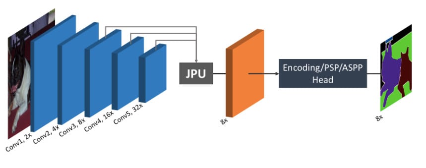
FastFCN —Fast Fully-connected network
Modern methods used to perform image segmentation use dilated convolutions at the core to extract high-resolution features. However, this approach requires a lot of computational power. To solve this issue, Huikai Wu, Junge Zhang, Kaiqi Huang, Kongming Liang and Yizhou Yu proposed a joint upsampling model known as Joint Pyramid Upsampling (JPU) which uses a joint upsampling method to extract high-resolution features. Therefore, reducing the time taken in computation while giving the best results, hence the name “Fast”.
The figure below shows its architecture.
You can implement this architecture in Tensorflow or Pytorch by following this link https://paperswithcode.com/paper/fastfcn-rethinking-dilated-convolution-in-the#code
Gated Shape CNNs for Semantic Segmentation (Gated-SCNN)
Gated-SCNN is an architecture used in semantic segmentation, it uses two-stream CNN where shape stream is added to the classical CNN architecture, and both are processed in parallel branches. Higher-level activations in the classical stream are used to gate lower level activation in the shape stream hence allowing the shape stream to focus on boundaries.
This architecture is unlike most image segmentation architectures where shape, color and texture are processed together on the deep CNN. You can implement this architecture through the GitHub link https://github.com/nv-tlabs/gscnn
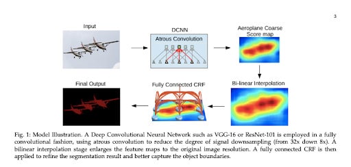
DeepLab
This architecture proposes three methods to be used in the task of semantic image segmentation which are:
- Atrous convolution which is convolution with upsampled filters – This allows us to control the resolution of computed features, it also allows us to enlarge filters field of view while maintaining parameters and computations.
- Atrous spatial pyramid pooling (ASPP) – This multiplies image objects into many scales then it captures objects and image context by using multiple sampling rates to probe the incoming convolutional feature layer.
- Combining Deep Convolutional Neural networks (DCNNs) and probabilistic graphical models to improve identifying object boundaries.
The figure below shows Deeplab architecture, source https://arxiv.org/abs/1606.00915
You can implement this architecture using Tensorflow “https://github.com/sthalles/deeplab_v3” or Pytorch “https://github.com/kazuto1011/deeplab-pytorch”,
You can also view and run this code on Google Colab https://colab.research.google.com/github/tensorflow/models/blob/master/research/deeplab/deeplab_demo.ipynb
Mask R-CNN
This architecture is used for instance image segmentation which extends Faster R-CNN (an architecture proposed by Shaoqing Ren et al to eliminate selective search and allow the network to learn region proposals) by adding an object mask predictor as a parallel branch to bounding box recognition.
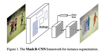
Source https://arxiv.org/abs/1703.06870
You can implement this architecture using Tensorflow “https://github.com/matterport/Mask_RCNN” or Pytorch “https://github.com/facebookresearch/detectron2”.
Image segmentation loss functions
An important component of neural networks is a loss function, it refers to a method of calculating prediction error (loss) in a neural network. While training a neural network, the loss is used to calculate gradients and eventually gradients are used to update weights. Libraries used in developing and training machine learning models i.e Tensorflow and Keras are packaged with inbuilt loss functions for performing specific objectives. These loss functions include Mean Squared Error (MSE), Binary Crossentropy (BCE), Categorical Crossentropy (CC), Sparse Categorical Crossentropy (SCC), etc.
Like other machine learning tasks, the Image segmentation task is affected directly by the choice of loss function because it controls the learning process. While Mean Squared Error (MSE) is specific for regression tasks, Image segmentation has loss functions specified for this task.
Image segmentation loss functions can be categorized into four categories: Distribution-based loss, Region-based loss, Boundary-based loss, and Compounded loss
These loss functions include:
Binary Cross-Entropy
Cross-entropy is a measure of the difference between two probability distributions for a given random variable or set of events. Cross entropy losses are very useful while performing classification tasks, hence very useful in classifying image pixels.
Binary cross-entropy loss computes the cross-entropy loss between true and predicted labels.
Binary Cross-Entropy is defined as:
LBCE(y, yˆ) = −(ylog(ˆy) + (1 − y)log(1 − yˆ))
Here, yˆ is the predicted value.
Importing binary cross-entropy in Tensorflow:
					import tensorflow as tf

tf.keras.losses.BinaryCrossentropy(
    from_logits=False, label_smoothing=0, reduction="auto", name="binary_crossentropy"
)
Weighted Binary Cross-Entropy
Weighted binary cross-entropy is a variant of Binary cross entropy which is used majorly when you have skewed or imbalanced data. Here, positive examples get weighted by some coefficient.
Weighted binary cross-entropy is defined as:
LW−BCE(y, yˆ) = −(β ∗ ylog(ˆy) + (1 − y)log(1 − yˆ))
To decrease the number of false negatives, set β>1. To decrease the number of false positives, set β<1.
Balanced Cross-Entropy
Balanced cross-entropy has similarities with weighted binary cross-entropy, the only difference is both positive and negative examples are weighted.
Balanced cross-entropy is defined as:
LBCE(y, yˆ) = −(β∗ylog(ˆy)+(1−β)∗(1−y)log(1−yˆ))
Here, β is defined as 1 − y H∗W
Sample implementation
					def balanced_cross_entropy(beta):
  def loss(y_true, y_pred):
    weight_a = beta * tf.cast(y_true, tf.float32)
    weight_b = (1 - beta) * tf.cast(1 - y_true, tf.float32)

    o = (tf.math.log1p(tf.exp(-tf.abs(y_pred))) + tf.nn.relu(-y_pred)) * (weight_a + weight_b) + y_pred * weight_b
    return tf.reduce_mean(o)

  return loss
Focal Loss
Focal loss is a variant of Binary cross-entropy which down-weights well-classified examples and enables the model to focus on learning hard examples. This model is useful while handling highly imbalanced classes like in Image Segmentation when the imbalance between background class and other classes is extremely high.
Below is the implementation of Focal loss in Tensorflow
					tfa.losses.SigmoidFocalCrossEntropy(
    from_logits: bool = False,
    alpha: tfa.types.FloatTensorLike = 0.25,
    gamma: tfa.types.FloatTensorLike = 2.0,
    reduction: str = tf.keras.losses.Reduction.NONE,
    name: str = 'sigmoid_focal_crossentropy'
)
Dice Loss
Dice Loss originated from the Dice coefficient which has been used to calculate the similarity of two images.
DL(y, pˆ) = 1 − (2ypˆ+ 1/ y + ˆp + 1)
One (1) is added in both the numerator and denominator to ensure that the function is not undefined in cases such as when y = 0 and ˆp = 0.
Intersection over Union (IoU)-balanced Loss
Intersection over Union (IoU)-balanced Loss increases localization accuracy of a model by increasing the gradient of samples with high IOU while decreasing the gradient of samples with low IOU
Below is the definition of IOU-balanced loss
IOU = TP/(TP+FP+FN)
Boundary loss
Boundary loss is that of a form of distance metrics on a space of contours, not regions. It, therefore, solved the issue of highly imbalanced segmentations because it uses integrals over the interface between regions instead of unbalanced integrals over the regions
Other loss functions that can be applied in image segmentation include Tversky Loss, Focal Tversky Loss, Sensitivity Specificity Loss, Shape-aware Loss, etc.
Image segmentation datasets
Generating your own data for research and educational purposes for image segmentation tasks can be quite a challenge. However, you shouldn’t worry about that because there are quite a number of open-source datasets that have already been created for this specific task. These Image datasets already have either semantic and instant segmentation defined.
Let’s discuss some of the most popular image segmentation datasets
COCO Dataset - Common Objects in Context
COCO is large-scale object detection, segmentation, and captioning dataset. It is a collection of everyday scenes containing segmented objects in their natural context. This dataset has photos of 91 objects that can be easily recognized and a total of 2.5 million labeled instances in 328k images. Source https://arxiv.org/abs/1405.0312 and https://cocodataset.org/#home
To download these images based on your preferred category, you can click here https://cocodataset.org/#download
You can perform a number of tasks from this dataset which include: object detections, keypoint detection, panoptic detection task, etc.
PASCAL Visual Object Classes (PASCAL VOC)
The PASCAL Visual Object Classes (VOC) dataset released in 2012 contains 20 different objects which include animals, households, vehicles, persons among others. The training and validation data has 11,530 images containing 27,450 ROI annotated objects and 6,929 segmentations.
To download this data, Go to http://host.robots.ox.ac.uk/pascal/VOC/voc2012/index.html#devkit, it’s a 2GB tar file
Open Images V6
Open Image v6 is a dataset of about 9 million images annotated with image-level labels, object segmentation masks, object bounding boxes, visual relationships, and localized narratives. The dataset is split into a training set of 9,011,219 images, a test set of 125,436 images, and a validation set of 41,620 images.
To download your preferred data subset, click here https://storage.googleapis.com/openimages/web/download.html
The Cityscapes Dataset
This dataset contains images of street scenes recorded in 50 different cities, with high-quality pixel-level annotations of 5,000 frames in addition to a larger set of 20,000 weakly annotated frames
Dataset is available for free for non-commercial usage, The dataset can be downloaded here https://www.cityscapes-dataset.com/downloads/
Other datasets include:
- The Cambridge-driving Labeled Video Database — CamVid
- The Oxford-IIIT Pet Dataset
Image segmentation frameworks & Tools
With recent advancements in computer vision, there are a number of both open source and closed source frameworks in different programming languages which allow you to take advantage of them and build an image segmentation model fast and efficiently.
Below are a few worth mentioning
TensorFlow Object Detection API – This is an open-source framework built on top of TensorFlow that makes it easy to develop, train and deploy object detection models. Here is the link to its GitHub repository https://github.com/tensorflow/models/tree/master/research/object_detection
DeepMask and SharpMask – DeepMask is an object proposal based on a convolutional neural network built by Facebook Research. Once the Algorithm is given an input patch, it will generate a class-agnostic mask and an associated score.
SharpMask on the other hand is an extension of DeepMask which generates higher-fidelity masks but implementing an additional top-down refinement step.
Fastai Visual Module – Fastai is an open-source python library that provides high-level components while giving the best results in deep learning domains. Fastai has a visual module that can be very helpful in handling image segmentation problems. Here is the link to its documentation https://docs.fast.ai/vision.core.html#Segmentation-masks
Opencv – Opencv is an open-source computer vision library written in C/C++ programming language with over 2500 optimized algorithms. Its main aim is to provide a real-time computer vision library.
Sefexa Image Segmentation Tool – Sefexa is a free software tool that can be installed on a windows computer and provides you with functionalities of image segmentation, analysis of images, and creation of ground truth.
Multipath network for Object Detection – Open source Torch framework developed by Facebook research to provide functionality to train Fast R-CNN and MultiPath Networks.
MIScnn – This is a python open-source library for medical image segmentation. It allows ease setting up pipelines with state-of-the-art convolutional neural networks and deep learning models.
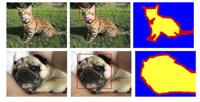
Image Segmentation in Python Using U-Net architecture
In this part of the tutorial, we are going to write python code using TensorFlow and U-net architecture to build a machine learning model for semantic image segmentation. The dataset that will be used for this tutorial is the Oxford-IIIT Pet Dataset, created by Parkhi et al. This dataset has 37 classes of pet images with 200 images for each class. All images have an associated ground truth annotation of breed, head ROI, and pixel-level trimap segmentation.
First, launch your Jupyter notebook or your favorite IDE, you can use Google Colab as well. Let’s start by installing TensorFlow examples using the pip command.
pip install -q git+https://github.com/tensorflow/examples.git
Let’s import the necessary libraries
					import tensorflow as tf
from tensorflow_examples.models.pix2pix import pix2pix
import tensorflow_datasets as tfds
from IPython.display import clear_output
import matplotlib.pyplot as plt
The dataset is already included in TensorFlow datasets which we have already imported. Version 3 of Oxford IIIT pet dataset contains segmentation masks which we will be using in this tutorial.
dataset, info = tfds.load('oxford_iiit_pet:3.*.*', with_info=True)
The following code performs image augmentation of flipping the images. Image augmentation is a technique in image processing that can be used to expand training datasets by modifying existing images, it’s an important technique since more data in machine learning means a better model is generated.
Another activity that we are going to perform is to normalize the images to [0,1] by dividing it by 255, also since segmentation masks are labelled as a set of {1, 2, 3}, we are going to subtract 1 to obtain {0, 1, 2} as a new masks set.
					def normalize(input_image, input_mask):
  input_image = tf.cast(input_image, tf.float32) / 255.0
  input_mask -= 1
  return input_image, input_mask
					@tf.function
def load_image_train(datapoint):
  input_image = tf.image.resize(datapoint['image'], (128, 128))
  input_mask = tf.image.resize(datapoint['segmentation_mask'], (128, 128))

  if tf.random.uniform(()) > 0.5:
    input_image = tf.image.flip_left_right(input_image)
    input_mask = tf.image.flip_left_right(input_mask)

  input_image, input_mask = normalize(input_image, input_mask)

  return input_image, input_mask
					def load_image_test(datapoint):
  input_image = tf.image.resize(datapoint['image'], (128, 128))
  input_mask = tf.image.resize(datapoint['segmentation_mask'], (128, 128))

  input_image, input_mask = normalize(input_image, input_mask)

  return input_image, input_mask
Since the dataset has already defined splits for train and test, let’s proceed and use them.
					TRAIN_LENGTH = info.splits['train'].num_examples
BATCH_SIZE = 64
BUFFER_SIZE = 1000
STEPS_PER_EPOCH = TRAIN_LENGTH // BATCH_SIZE
					train = dataset['train'].map(load_image_train, num_parallel_calls=tf.data.AUTOTUNE)
test = dataset['test'].map(load_image_test)
					train_dataset = train.cache().shuffle(BUFFER_SIZE).batch(BATCH_SIZE).repeat()
train_dataset = train_dataset.prefetch(buffer_size=tf.data.AUTOTUNE)
test_dataset = test.batch(BATCH_SIZE)
Let’s pick an image from the dataset with their corresponding segmentation mask and display using matplotlib imshow method.
					def display(display_list):
  plt.figure(figsize=(15, 15))

  title = ['Input Image', 'True Mask', 'Predicted Mask']

  for i in range(len(display_list)):
    plt.subplot(1, len(display_list), i+1)
    plt.title(title[i])
    plt.imshow(tf.keras.preprocessing.image.array_to_img(display_list[i]))
    plt.axis('off')
  plt.show()
					for image, mask in train.take(3):
  sample_image, sample_mask = image, mask
display([sample_image, sample_mask])
Regardless of the image you select, you will get an output with an image and its mask as shown below.
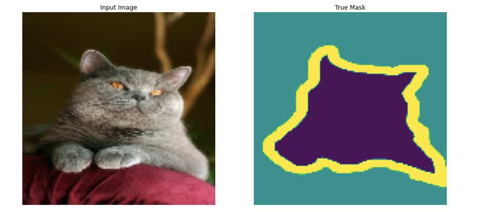
Let’s define our modified U-Net architecture model, as discussed earlier, U-Net consists of an encoder (downsampler) and decoder (upsampler)
Since each pixel can be classified into either of the three classes (pixels belonging to the pet, pixels belonging to the boundary, and another one pixel which is the background), we are going to define output channels as 3.
OUTPUT_CHANNELS = 3
We are going to use MobileNetv2 which is a pre-trained model as an encoder so as to learn robust features and reduce the number of trainable parameters. MobileNetV2 model which is prepared and ready to use in tf.keras.applications. Encoders consist of outputs from intermediate layers and from this example, we will not be training our encoder.
					base_model = tf.keras.applications.MobileNetV2(input_shape=[128, 128, 3], include_top=False)

# Use the activations of these layers
layer_names = [
    'block_1_expand_relu',   # 64x64
    'block_3_expand_relu',   # 32x32
    'block_6_expand_relu',   # 16x16
    'block_13_expand_relu',  # 8x8
    'block_16_project',      # 4x4
]
base_model_outputs = [base_model.get_layer(name).output for name in layer_names]

# Create the feature extraction model
down_stack = tf.keras.Model(inputs=base_model.input, outputs=base_model_outputs)

down_stack.trainable = False
The decoder or upsampler is a series of upsample blocks, and from this tutorial, you will use pix2pix upsample found in TensorFlow examples.
					up_stack = [
   pix2pix.upsample(512, 3),  # 4x4 -> 8x8
   pix2pix.upsample(256, 3),  # 8x8 -> 16x16
   pix2pix.upsample(128, 3),  # 16x16 -> 32x32
   pix2pix.upsample(64, 3),   # 32x32 -> 64x64
]
Next, let’s define a U-Net model
					def unet_model(output_channels):
  inputs = tf.keras.layers.Input(shape=[128, 128, 3])

  # Downsampling through the model
  skips = down_stack(inputs)
  x = skips[-1]
  skips = reversed(skips[:-1])

  # Upsampling and establishing the skip connections
  for up, skip in zip(up_stack, skips):
    x = up(x)
    concat = tf.keras.layers.Concatenate()
    x = concat([x, skip])

  # This is the last layer of the model
  last = tf.keras.layers.Conv2DTranspose(
      output_channels, 3, strides=2,
      padding='same')  #64x64 -> 128x128

  x = last(x)

  return tf.keras.Model(inputs=inputs, outputs=x)
Compile and train our model
Since the network is trying to assign each pixel a label, that means each pixel will be assigned either of the set {0, 1, 2}, for this case the best loss function to implement while compiling the model is Sparse Cross-entropy with logits which is found in Keras loss method losses.SparseCategoricalCrossentropy(from_logits=True).
Let’s compile the mode
					model = unet_model(OUTPUT_CHANNELS)
model.compile(optimizer='adam',
              loss=tf.keras.losses.SparseCategoricalCrossentropy(from_logits=True),
              metrics=['accuracy'])
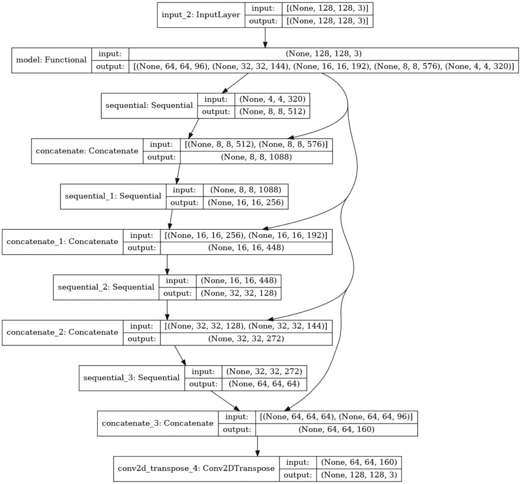
You can take advantage of Keras utility function known as `plot_model()` method to display the structure of our model.
tf.keras.utils.plot_model(model, show_shapes=True)
Output
Next, let’s see what the model predicts before you initiate its training.
					def create_mask(pred_mask):
  pred_mask = tf.argmax(pred_mask, axis=-1)
  pred_mask = pred_mask[..., tf.newaxis]
  return pred_mask[0]
					def create_mask(pred_mask):
  pred_mask = tf.argmax(pred_mask, axis=-1)
  pred_mask = pred_mask[..., tf.newaxis]
  return pred_mask[0]
show_predictions()
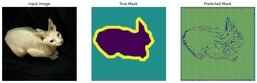
Finally, let’s start training the model and using the Keras callback method you will display the predicted image mask after every epoch. This will help evaluate how the model is performing after every epoch.
					class DisplayCallback(tf.keras.callbacks.Callback):
  def on_epoch_end(self, epoch, logs=None):
    clear_output(wait=True)
    show_predictions()
    print ('\nSample Prediction after epoch {}\n'.format(epoch+1))
EPOCHS = 20
VAL_SUBSPLITS = 5
VALIDATION_STEPS = info.splits['test'].num_examples//BATCH_SIZE//VAL_SUBSPLITS

model_history = model.fit(train_dataset, epochs=EPOCHS,
                          steps_per_epoch=STEPS_PER_EPOCH,
                          validation_steps=VALIDATION_STEPS,
                          validation_data=test_dataset,
                          callbacks=[DisplayCallback()])
You will notice an improvement of the model prediction after each epoch and that means the more you train, the better the model.
Let’s use the model you have built to make predictions and let’s see how it performs.
show_predictions(test_dataset, 2)
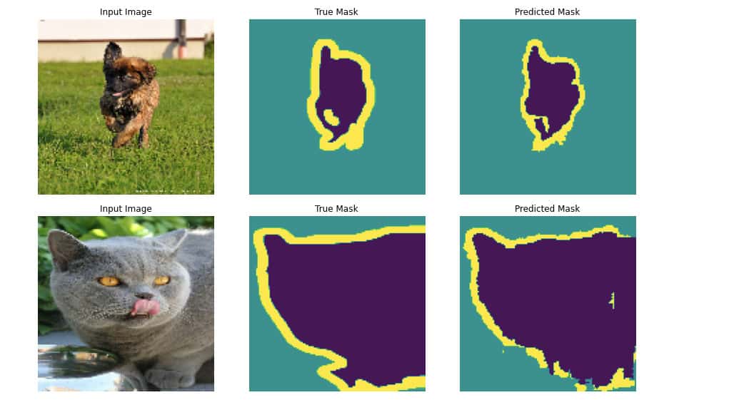
The results are impressive since the model is doing pretty well in labeling the pixel.
Implementing Mask R-CNN for Image Segmentation with Python
In this tutorial, you will implement Mask R-CNN architecture in python using the Tensorflow library.
Let’s start by cloning Mask R-CNN for TensorFlow Version 2+
git clone https://github.com/IgnacioAmat/Mask_RCNN.git
Next step, create a .py or .ipynb, and let’s import the required libraries.
					import os
import sys
import skimage.io
import matplotlib
import matplotlib.pyplot as plt
from mrcnn import utils
import mrcnn.model as modellib
from mrcnn import visualize
import coco
Next step is defining all the directories that you will use in this tutorial.
					# Root directory of the project
ROOT_DIR = os.path.abspath("./")
sys.path.append(ROOT_DIR)  # To find local version of the library
# Import COCO config
sys.path.append(os.path.join(ROOT_DIR, "coco/"))  # To find local version
# Directory to save logs and trained model
MODEL_DIR = os.path.join(ROOT_DIR, "logs")
Let’s define the path where the trained weights for COCO dataset weights, and initiate download if the weights are not available.
					# Local path to trained weights file
COCO_MODEL_PATH = os.path.join(ROOT_DIR, "mask_rcnn_coco.h5")
# Download COCO trained weights from Releases if needed
if not os.path.exists(COCO_MODEL_PATH):
    utils.download_trained_weights(COCO_MODEL_PATH)
# Directory of images to run detection on
IMAGE_DIR = os.path.join(ROOT_DIR, "images")
Now let’s create an inference class that will be used to infer the Mask R-CNN model
					class InferenceConfig(coco.CocoConfig):
    # Set batch size to 1 since we'll be running inference on
    # one image at a time. Batch size = GPU_COUNT * IMAGES_PER_GPU
    GPU_COUNT = 1
    IMAGES_PER_GPU = 1
config = InferenceConfig()
config.display()
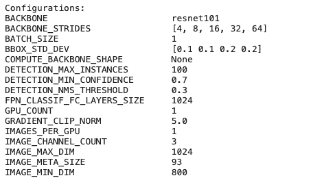
This will output a number of configurations for our model including backbone as Resnet101, Resnet101 is a convolutional neural network that is 101 layers deep.
Create a model object in inference mode and load weights trained using the Ms-COCO dataset.
					model = modellib.MaskRCNN(mode="inference", model_dir=MODEL_DIR, config=config)
model.load_weights(COCO_MODEL_PATH, by_name=True)
Define class names
					class_names = ['BG', 'person', 'bicycle', 'car', 'motorcycle', 'airplane',
               'bus', 'train', 'truck', 'boat', 'traffic light',
               'fire hydrant', 'stop sign', 'parking meter', 'bench', 'bird',
               'cat', 'dog', 'horse', 'sheep', 'cow', 'elephant', 'bear',
               'zebra', 'giraffe', 'backpack', 'umbrella', 'handbag', 'tie',
               'suitcase', 'frisbee', 'skis', 'snowboard', 'sports ball',
               'kite', 'baseball bat', 'baseball glove', 'skateboard',
               'surfboard', 'tennis racket', 'bottle', 'wine glass', 'cup',
               'fork', 'knife', 'spoon', 'bowl', 'banana', 'apple',
               'sandwich', 'orange', 'broccoli', 'carrot', 'hot dog', 'pizza',
               'donut', 'cake', 'chair', 'couch', 'potted plant', 'bed',
               'dining table', 'toilet', 'tv', 'laptop', 'mouse', 'remote',
               'keyboard', 'cell phone', 'microwave', 'oven', 'toaster',
               'sink', 'refrigerator', 'book', 'clock', 'vase', 'scissors',
               'teddy bear', 'hair drier', 'toothbrush']
Load your test image and use the model build to detect image objects.
					image = skimage.io.imread(os.path.join(IMAGE_DIR, 'elephant.jpg'))
results = model.detect([image], verbose=1)
Finally, visualize your results
					r = results[0]
visualize.display_instances(image, r['rois'], r['masks'], r['class_ids'],
                            class_names, r['scores'])
Output
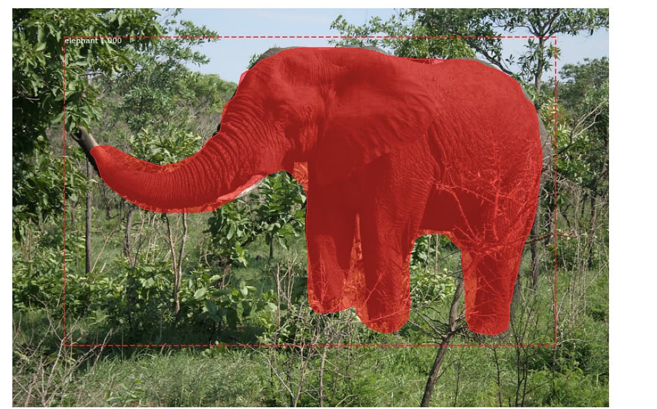
Since my test image has an Elephant, the model was able to map the location of the Elephant object in the image and also indicate that it is an Elephant. You can test this model with different images and see how your model performs.
Final Thoughts
Image segmentation is a very important field in Computer vision as it enables the advancement of critical technologies including Self-driving cars and improvement in the accuracy of medical images, machines can detect diseases faster and more accurately among other advantages.
The computer vision market value is expected to reach USD 19.1 billion by 2027, according to a report by Grand View Research, Inc. Image segmentation being one of the 5 major topics in computer vision, as an AI professional it is very important to learn this topic in order to participate in the research and growth of this technology.
Helpful Resources
From all the topics and sub-topics that we’ve covered on image segmentation, you now have enough information to get started and dive deep into this topic. Below are some helpful links to resources that can help you dive deeper.
- CS231n Convolutional Neural Networks for Visual Recognition http://cs231n.stanford.edu/
- A Simple Guide to Semantic Segmentation https://www.topbots.com/semantic-segmentation-guide/
- Semantic Segmentation in the era of Neural Networks https://theaisummer.com/Semantic_Segmentation/
- Semantic Segmentation: Wiki, Applications and Resources https://www.kdnuggets.com/2018/10/semantic-segmentation-wiki-applications-resources.html
Coursera image segmentation https://www.coursera.org/lecture/deep-learning-in-computer-vision/image-segmentation-o5e7h