
Table of Contents
Introduction to Gradient Clipping Techniques with Tensorflow
Deep neural networks are prone to the vanishing and exploding gradients problem. This is especially true for Recurrent Neural Networks (RNNs). RNNs are mostly applied in situations where short-term memory is needed. For instance, when translating to certain languages such a French it’s important to understand the gender of preceding words. For example, translating the sentence “The boy jumped over the fence” would result in “Le garçon a sauté par-dessus la clôture”. If you change boy to girl the resulting translation becomes “La fille a sauté par-dessus la clôture”.

In this case, a neural network would need to keep track the context of who is jumping over the fence to make the right translation. This is also applicable when classifying the sentiment of a sentence because certain words are positive while others are negative. Therefore, the network has to understand how the word is used in the whole sentence to determine its polarity. RNNs majorly deal with sequence data. Therefore, backpropagation happens through time.
Since the networks are usually deep, the weights are updated at various intervals. The weights could tend to disappear through time leading to vanishing gradients or they could become too large leading to the exploding gradients problem. In this article, let’s explore these problems and their possible solutions.
Common problems with backpropagation
The cost function or error in an RNN is computed at every time point t. During the training process, errors are reduced via gradient descent. This is done by figuring out the place where the error is at a minimum. Gradient descent adjusts the errors by reducing the cost function. The error at time step t is represented by Et in the unrolled RNN as shown in the image below. The error is calculated by comparing the expected output and the network’s output.
Forward pass & backward pass
The error computed at time t needs to be propagated back to the network so that it can improve its performance. The propagation happens through time i.e the weights and biases are updated at each time step. Backpropagation computes the gradients of the cost function with respect to the cost function and the biases.
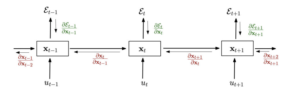
Source. An example of an unrolled RNN
The number of time steps depends on the design of your network. Remember that weights are initialized to very small numbers closer to zero at the beginning. These weights are updated during the backpropagation process. When these small weights are multiplied by small gradients, the result is even smaller weights. This means that the network is updated with very tiny weights and hence learns very slowly. The small weights then result in small gradients during the forward propagation. This results in the gradients decreasing gradually. At a certain point, the gradient can become zero. This is referred to as the vanishing gradients problem. The result of this is a useless network that cannot be used in practice.
So far we have talked about situations where the weights become too small leading to very small gradients. In other scenarios, the weights could become so large resulting in enormous gradients. This is referred to as the exploding gradients problem.
The vanishing gradients and exploding gradients problems can be addressed by scaling the gradients and clipping gradients that are above or below a certain threshold. This is usually referred to as gradient clipping.
What causes exploding gradients?
Huge updates in network gradient will usually result in NANs in the model weights. Such a network will also predict NANs for all values. The exploding gradient problem can be caused by:
- Choosing the wrong learning rate which leads to huge updates in the gradients
- Failing to scale a data set leading to very large differences between data points
- Applying a loss function that computes very large error values
How to identify and catch exploding gradients?
It is possible to identify exploding gradients when you start the process of training your network. This is especially crucial for deep recurrent networks and LSTMs. You can catch the exploding gradients by weaving proper logging mechanisms into your model’s training process. For instance, you can:
- Log the model’s loss
- Create triggers to notify you of sudden jumps in the model loss
One tool that you can use to monitor your model’s loss is TensorFlow’s TensorBoard.
How to fix exploding gradients
In this article, we’ll focus on how exploding gradients can be addressed using gradient clipping. However, it is worth mentioning other alternatives. These potential solutions involve solving the problems mentioned above, by:
- Choosing the appropriate loss function
- Ensuring that the training data is standardized
- Choosing a small learning rate so that there are no large updates in the gradients
- Using Long Short Term Memory (LSTMS) which is more adapted to tackling this problem
- L2 Regularization that involves penalizing the network for large weight values
That said, LSTMs are still prone to exploding gradients. It’s, therefore, important to look at how this problem can be addressed by gradient clipping.
What is Gradient Clipping and how does it occur?
Gradient clipping involves capping the error derivatives before propagating them back through the network. The capped gradients are used to update the weights hence resulting in smaller weights. The gradients are capped by scaling and clipping. Gradient clipping involves forcing the gradients to a certain number when they go above or below a defined threshold.
Types of Clipping techniques
Gradient clipping can be applied in two common ways:
- Clipping by value
- Clipping by norm
Let’s look at the differences between the two.
Gradient Clipping-by-value
Clipping the gradient by value involves defining a minimum and a maximum threshold. If the gradient goes above the maximum value it is capped to the defined maximum. Similarly, if the gradient goes below the minimum it is capped to the stated minimum value.
Gradient Clipping-by-norm
Clipping the gradient by norm ensures that the gradient of every weight is clipped such that its norm won’t be above the specified value. According to this blog:
“…a norm is a function that accepts as input a vector from our vector space V and spits out a real number that tells us how big that vector is. ”
Gradient clipping in deep learning frameworks
You are now familiar with exploding gradients and how to solve it. Let’s now take a look at how gradient clipping can be applied in deep learning frameworks.
How to avoid exploding gradients with gradient clipping
Gradient clipping is applied differently from one framework to another. However, as you shall see the underlying principles are the same. Let’s now walk through a couple of examples of how you can clip gradients in deep learning models.
Gradient Clipping in Keras
Applying gradient clipping in TensorFlow models is quite straightforward. The only thing you need to do is pass the parameter to the optimizer function. All optimizers have a `clipnorm` and a `clipvalue` parameters that can be used to clip the gradients.
Let’s look at clipping the gradients using the `clipnorm` parameter using the common MNIST example.
import tensorflow as tf
from tensorflow.keras.datasets import mnist
(x_train, y_train), (x_test, y_test) = mnist.load_data()
x_train, x_test = x_train / 255., x_test / 255.
model = tf.keras.models.Sequential([
tf.keras.layers.Flatten(input_shape=(28, 28)),
tf.keras.layers.Dense(128,activation='relu'),
tf.keras.layers.Dense(10)
])
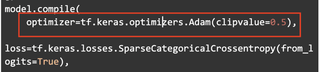
model.compile(
optimizer=tf.keras.optimizers.Adam(clipvalue=0.5),
loss=tf.keras.losses.SparseCategoricalCrossentropy(from_logits=True),
metrics=[tf.keras.metrics.SparseCategoricalAccuracy()],
)
Clipping by value is done by passing the `clipvalue` parameter and defining the value. In this case, gradients less than -0.5 will be capped to -0.5, and gradients above 0.5 will be capped to 0.5.
The `clipnorm` gradient clipping can be applied similarly. In this case, 1 is specified.
					model.compile(
    optimizer=tf.keras.optimizers.Adam(clipnorm=1.0),
    loss=tf.keras.losses.SparseCategoricalCrossentropy(from_logits=True),
    metrics=[tf.keras.metrics.SparseCategoricalAccuracy()],
)
This means that when the vector norm of a gradient goes beyond 1, the values of that vector will be rescaled in such a way that the norm of the vector equals 1.

Gradient Clipping in TensorFlow
Keras is the official high-level API for building models in TensorFlow. It is also the easiest and most popular way to build neural networks. However, you can still apply gradient clipping if you are building your networks without using TensorFlow. To apply gradient clipping in TensorFlow, you’ll need to make one little tweak to the optimization stage.
The gradients are computed using the `tape.gradient` function. After obtaining the gradients you can either clip them by norm or by value. Here’s how you can clip them by value.
gradients = [(tf.clip_by_value(grad, clip_value_min=-1.0, clip_value_max=1.0)) for grad in gradients]
Clipping by norm can be done in a similar fashion.
gradients = [(tf.clip_by_norm(grad, clip_norm=2.0)) for grad in gradients]
The complete optimization function would look like this:
					optimizer = tf.optimizers.Adam()
def optimize(x, y):
    with tf.GradientTape() as tape:
        predictions = network(x, is_training=True)
        loss = cross_entropy_loss(predictions, y)
    gradients = tape.gradient(loss, model.trainable_variables)
    gradients = [(tf.clip_by_value(grad, clip_value_min=-1.0, clip_value_max=1.0)) for grad in gradients]
    optimizer.apply_gradients(zip(gradients,     model.trainable_variables))
Regression predictive modeling problem
Let’s now investigate the effect of gradient clipping using a regression problem. The first step is to obtain a regression dataset. A regression dataset can be generated using Scikit-learn.
from sklearn.datasets import make_regression
X, y = make_regression(n_samples=10000, n_features=30, random_state=65)
Next, split the dataset into a training set and a validation set. Let’s use 20% of the data for testing and the rest for training.
					from sklearn.model_selection import train_test_split
X_train, X_test, y_train, y_test = train_test_split(
    X, y, test_size=0.20)
The next step is to define the network. A simple network with 2 Dense layers will suffice here. You can compile the network with your preferred optimizer. Let’s use the common Adam optimizer here. After that, train and evaluate the network.
					regressor1 = tf.keras.models.Sequential([
  tf.keras.layers.Dense(35,input_dim=30,activation='relu',),
  tf.keras.layers.Dense(1,activation='linear')
])
regressor1.compile(loss='mean_squared_error', optimizer=tf.keras.optimizers.Adam())
regressor1.fit(X_train, y_train,validation_data=(X_test, y_test),epochs=30)
regressor1.evaluate(X_test, y_test)
Note the loss toward the end of the network training as well as the loss after evaluation. Later, we’ll compare these results after clipping the gradient.
Multilayer perceptron with exploding gradients
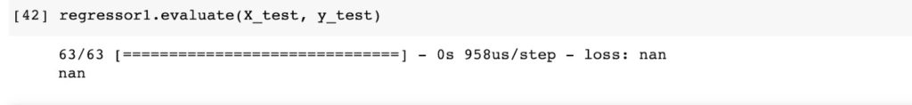
A great way to illustrate exploding gradients is to make the X and y values into very large numbers. For instance, raising them a certain power. In such a case you will realize that the loss becomes nan. If the values are too large the loss becomes infinite.
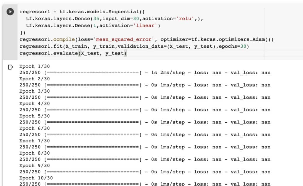
The result will also be nan on evaluating this kind of network. Needless to say, such a network is useless.
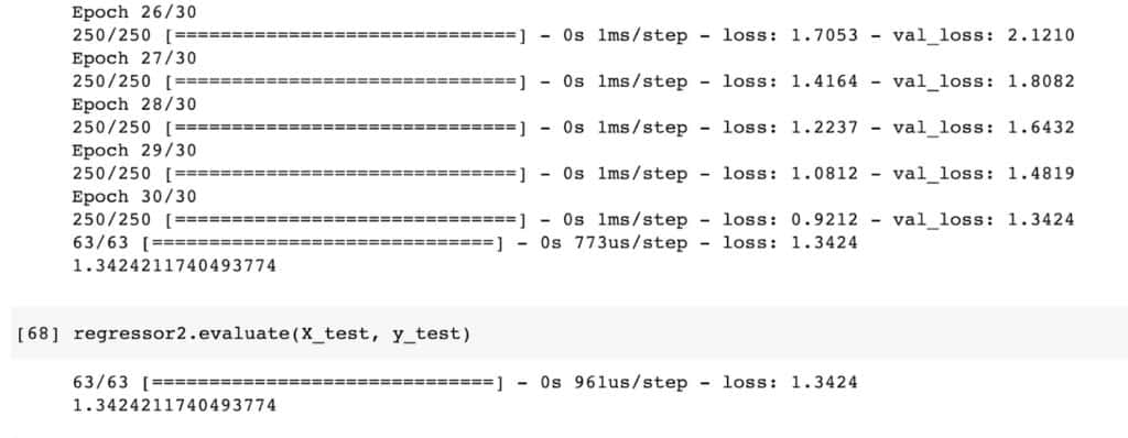
MLP with gradient norm scaling
Let’s now apply gradient by norm to the network and observe how that compares to the network without. The gradients can be clipped by passing the `clipnorm` to the Adam optimizer. In this case, the gradients are rescaled to a vector norm of 1.
					regressor2 = tf.keras.models.Sequential([
  tf.keras.layers.Dense(35,input_dim=30,activation='relu',),
  tf.keras.layers.Dense(1,activation='linear')
])
regressor2.compile(loss='mean_squared_error', optimizer=tf.keras.optimizers.Adam(clipnorm=1))

regressor2.fit(X_train, y_train,validation_data=(X_test, y_test),epochs=30)
regressor2.evaluate(X_test, y_test)
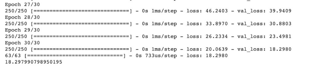
Let’s look at the weights of the last few epochs as well as the error after evaluating the network. It is evident that the loss is much lower compared to the network whose gradients haven’t been clipped.
MLP with gradient value clipping
Let’s repeat the above process but now clip the gradients by value. That is done using the `clipvalue` argument. In this case a maximum value of 3 is dictated. This will clip gradients above 3 to 3 and gradients below -3 to 3.
					regressor3 = tf.keras.models.Sequential([
  tf.keras.layers.Dense(35,input_dim=30,activation='relu',),
  tf.keras.layers.Dense(1,activation='linear')
])
regressor3.compile(loss='mean_squared_error', optimizer=tf.keras.optimizers.Adam(clipvalue=3))
regressor3.fit(X_train, y_train,validation_data=(X_test, y_test),epochs=30)
regressor3.evaluate(X_test, y_test)
Here is the training and validation loss of this network.
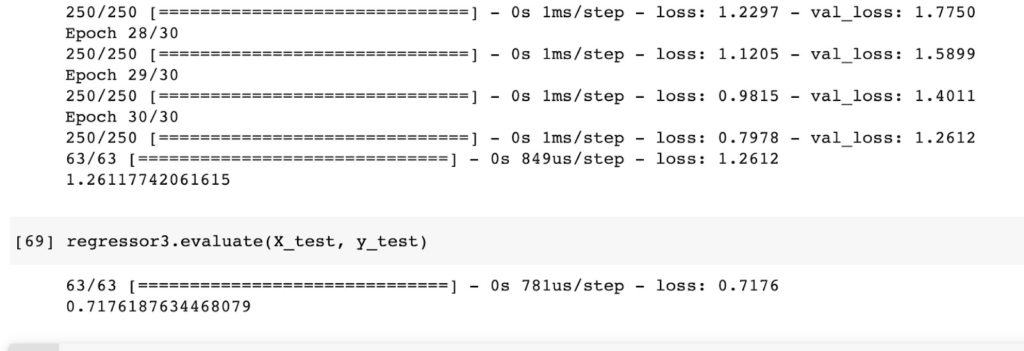
As seen above the loss is much lower compared to the other network where gradient clipping wasn’t implemented.
It is, however, important to mention that gradient clipping is not a solution to failure to perform proper data preprocessing such as scaling the data. In fact, in such scenarios clipping the gradients might not work. You will have to address the root cause of the exploding gradients.
Gradient Clipping in PyTorch
Let’s now look at how gradients can be clipped in a PyTorch classifier. The process is similar to TensorFlow’s process, but with a few cosmetic changes. Let’s illustrate this using this CIFAR classifier.
Let’s start by loading and transforming the data. The data can be loaded easily using `torchvision`.
					import torch
import torchvision
import torchvision.transforms as transforms
transform = transforms.Compose(
    [transforms.ToTensor(),
     transforms.Normalize((0.5, 0.5, 0.5), (0.5, 0.5, 0.5))])

batch_size = 4

trainset = torchvision.datasets.CIFAR10(root='./data', train=True,
                                        download=True, transform=transform)
trainloader = torch.utils.data.DataLoader(trainset, batch_size=batch_size,
                                          shuffle=True, num_workers=2)

testset = torchvision.datasets.CIFAR10(root='./data', train=False,
                                       download=True, transform=transform)
testloader = torch.utils.data.DataLoader(testset, batch_size=batch_size,
                                         shuffle=False, num_workers=2)

classes = ('plane', 'car', 'bird', 'cat',
           'deer', 'dog', 'frog', 'horse', 'ship', 'truck')
Next, let’s define the convolutional neural network.
					import torch.nn as nn
import torch.nn.functional as F
class Net(nn.Module):
    def __init__(self):
        super().__init__()
        self.conv1 = nn.Conv2d(3, 6, 5)
        self.pool = nn.MaxPool2d(2, 2)
        self.conv2 = nn.Conv2d(6, 16, 5)
        self.fc1 = nn.Linear(16 * 5 * 5, 120)
        self.fc2 = nn.Linear(120, 84)
        self.fc3 = nn.Linear(84, 10)

    def forward(self, x):
        x = self.pool(F.relu(self.conv1(x)))
        x = self.pool(F.relu(self.conv2(x)))
        x = x.view(-1, 16 * 5 * 5)
        x = F.relu(self.fc1(x))
        x = F.relu(self.fc2(x))
        x = self.fc3(x)
        return x

net = Net()
The next step is to define the network’s optimizer and loss function.
					import torch.optim as optim

criterion = nn.CrossEntropyLoss()
optimizer = optim.SGD(net.parameters(), lr=0.001, momentum=0.9)
The next move is to train the network. This is the stage where the gradient clipping is defined. The magic is done by this single line of code when clipping the gradient by value.
nn.utils.clip_grad_value_(net.parameters(), clip_value=1.0)
When clipping the gradient by norm this line would look like this.
nn.utils.clip_grad_norm_(model.parameters(), max_norm=2.0, norm_type=2)
Here’s how the entire training loop looks like for reference.
					for epoch in range(2):  # loop over the dataset multiple times


    running_loss = 0.0
    for i, data in enumerate(trainloader, 0):
        # get the inputs; data is a list of [inputs, labels]
        inputs, labels = data

        # zero the parameter gradients
        optimizer.zero_grad()

        # forward + backward + optimize
        outputs = net(inputs)
        loss = criterion(outputs, labels)
        loss.backward()
        nn.utils.clip_grad_value_(net.parameters(), clip_value=1.0)
        optimizer.step()

        # print statistics
        running_loss += loss.item()
        if i % 2000 == 1999:    # print every 2000 mini-batches
            print('[%d, %5d] loss: %.3f' %
                  (epoch + 1, i + 1, running_loss / 2000))
            running_loss = 0.0

print('Finished Training')
Why gradient clipping accelerates training
You have already seen the gradient clipping is very important in deep Recurrent Networks because they are more prone to the vanishing gradients problem. At the very least, clipping the gradients will ensure that you obtain a model that doesn’t predict all NANs. However, how exactly does gradient clipping accelerate model training? Clipping the gradients makes training faster by enabling the model to converge faster. This is to say that the training arrives at a minimum error faster. Exploding gradients makes the error diverge hence a global or local minima is not achieved. Clipping the exploding gradients forces the errors to start converging to a minimum point.
Final thoughts
n this article, you’ve gained an intuitive understanding of the vanishing and exploding gradient problem and how to address them. You’ve also learned some of the reasons that can lead to the occurrence of vanishing and exploding gradient problems. More specifically, you have learned:
- What causes exploding gradients?
- How to identify exploding gradients
- How to fix exploding gradients
- What is gradient clipping
- How to clip gradients in TensorFlow
- Applying gradient clipping in PyTorch