
Landscape of Data
Data history is a long story detailing the evolution of data collection, storage, and processing. When reading this article, it should be worth noting that a vast amount of data surrounds us. These data are growing exponentially due to technological advancements in processing power, storage, and connectivity.
A recent report from the World Economic Forum gives us a glimpse of the enormous amount of data created, and the reports point out that:
“Around 2.5 quintillion bytes of data are created every single day One of the most significant sources of this data is consumers, whose online browsing, past purchases and payments leave huge trails of information.”
The report also highlights in its infographics that:
- 500 million tweets are sent
- 294 billion emails are sent
- 4 Petabytes of data are made on Facebook
- 65 billion messages are sent on WhatsApp
- 5 billion searches are done
The report forecasts that by 2025, daily data creation globally should grow exponentially to 463 exabytes of data. These data are not created equal as their source varies widely but can be grouped as either be structured or unstructured. Structured data is quantitative data that consists of numbers and values that fit neatly within fixed fields and columns. In contrast, Unstructured data is qualitative data that consists of audio, images, videos, descriptions, social media posts, etc. Also, the differentiating factor is the defined pattern inherent in data, as structured data patterns are easily searchable. In contrast, the unstructured data pattern is not easily searchable. The methods of collecting, preprocessing, and analyzing these two types of data differ and depend on the data format.
It is essential to know how these data we speak of are being captured and saved. They are currently the most valuable commodity in the world. The database is an organized collection of data that provides methods to access and manipulate data. We have five(5) specific databases for various use cases based on the structured and unstructured data types.
- Relational model database: Data is stored in related tables as rows and columns; examples include PostgreSQL, IBM Db2.
- Document model database: Data is stored in JSON-like documents, rather than rows and columns; examples include MongoDB, Firebase.
- Key-value model database: Data is stored as an attribute name(key) with its corresponding value; examples include Redis, DynamoDB
- Graph model database: Data is stored in values and connection; examples include Neo4j, JanusGraph
- Wide-Columnar model database: Wide-column stores structure data around columns rather than rows; examples include Google Cloud BigTable, Apache Cassandra.
With data efficiently stored, the next step will be to make sense out of this data. Carly Fiorina pointed out that “the goal is to turn data into information, and information into insights.” This transformation can not be over-emphasized as information extraction. Knowledge discovery is now necessary for data to be valuable, leading to Data Mining.
Before we further into Data Mining, it is pertinent to clarify the difference between data and dataset. Data are facts, observations, and statistics (unprocessed and processed) collected together for reference or analysis. At the same time, a dataset is a collection of data associated with a unique body of work.
What is Data Mining?
The definition of Mining from Wikipedia is “the extraction of valuable minerals or other geological materials from the Earth.” This statement implies that the term “data mining” is a misnomer because it is not an extraction of data but an extraction of patterns and knowledge from data.
Data Mining is about solving problems by exploring and analyzing data present in the database to glean meaningful patterns and trends. It is an interdisciplinary field of science and technology with an overall goal to discover already present unknown patterns for data. Escalating these identified valid patterns into helpful information and transforming the information into an understandable structure for further use. Data Mining is dependent on data collection, warehousing, and processing.
It is often taken that Data Mining is synonymous with Knowledge Discovery in Database (KDD) processes. Data Mining is the analysis step in the Knowledge Discovery in Database (KDD) process. Based on the Cross-industry standard process for data mining (CRISP-DM), we have six(6) divisions:
- Business understanding and goal identification: This is the first phase of a data mining project that involves exploring and analyzing the application domain and getting the essential problem specifications from a business perspective. This step consists of obtaining and understanding domain experts’ requirements, defining final objectives curated with the end-users in mind, and using this knowledge to build a data mining problem definition and a preliminary plan to achieve the given goals.
- Data understanding: This is the comprehension of data which includes sourcing of the data, exploring the data to deduct some familiarity and identify data quality problems, discovering first insights from the data, and probably form a hypothesis about hidden patterns from intersecting subsets of the data. This phase involves exploring the data and determining how well it addresses the business problems and needs. This phase checks for data sufficiency if additional data is needed or some subsets need to be removed.
- Data Preparation: This phase includes operations for data cleaning, data integration, data transformation, and data reduction. This phase is synonymous with data preprocessing. It was previously stated that data mining depends on efficient processing. Thus, before utilizing the various data mining classes and respective algorithms, assembling a target set is required. This target set is the data set fed to the model, which significantly improves the initial raw data. Data preparation tasks are fitting to be multiple times and not any prescribed order; this phase can remarkably improve the insight and information discovered through data mining, hence is the most essential and most extended step in the workflow.
- Modeling: This is the essential phase where various data mining classes and respective algorithms are carried out to extract valid data patterns. These data mining classes will extensively be explained in the next section. This phase selects and applies a variety of modeling techniques and tunes algorithm parameters to yield optimal results. Some of these modeling techniques have specific requirements from the data and occasionally lead to stepping back to the data preparation to implement them.
- Evaluation: Typically, several modeling techniques can be applied to the same data mining problem type, so it is pertinent to estimate, interpret and judge the mined patterns based on precisely defined performance metrics. This phase results in the decision-making on the various data mining results by evaluating models, reviewing steps carried out to construct the models, and, most importantly, its alignment to the project (business) objectives.
- Deployment: After adequate evaluation, this last phase involves using the knowledge discovered, incorporating the various systems for other processes, or reporting via visualizations. This phase organizes the results of data mining.
Data mining involves six(6) standard classes of tasks.
- Regression: Regression is an instance of supervised learning (a training set of correctly identified observations is available) where statistical processes are used for estimation tasks. It estimates the relationship between the target variable (dependent/outcome variable) and one or more predictors ( independent variables/features). It aids the prediction of continuous outcomes. Regressions can be either linear or nonlinear. They can be modeled by an equation of a straight line and various curve functions, respectively. These different modeling functions has yielded quite a several regression analysis listed below but not limited to:
- Linear Regression
- Logistic Regression
- Polynomial Regression
- Ridge Regression
- Lasso Regression
- Stepwise Regression
- Poisson Regression
- Quasi Poisson Regression
- ElasticNet Regression
- Bayesian Regression
- Robust Regression
- Ecological Regression
- Tobit Regression
- Quantile Regression
- Cox Regression
- Negative Binomial Regression
- Ordinal Regression
- Support Vector Regression
- Partial Least Square (PLS) Regression
- Principal Component Regression
The list is quite exhaustive; it is not imperative to know all the various techniques. They depend on the type of data and distribution. It is worth noting that these regression algorithms are designed for multiple types of analysis.
- Classification: This is also an instance of supervised learning. A set of statistical processes is used to identify where a new observation belongs to a group of defined and known categories (subpopulation/classes). It is a predictive modeling process that separates data into multiple categorical classes based on known labels. Classification tasks based on the various formats they might appear can be:
- Binary Classification
- Multi-class Classification
- Multi-label Classification
- Imbalance Classification
The various classification algorithms to aid proceeding in any of the classification tasks are but not limited to:
- Logistic Regression
- Naive Bayes
- Stochastic Gradient Descent
- K-Nearest Neighbor
- Decision Tree
- Random Forest
- Artificial Neural Network
- Support Vector Machine
- Clustering: Clustering: This is an instance of unsupervised learning (a training set without labels) that determines the intrinsic grouping of data based on similarity and similarity between them based on calculating multivariate distances. It involves collecting data points into natural groups or clusters when it appears there is no class information to be predicted. There are no clear criteria for these groupings as it is subjected to the user’s choice. There are various clustering methods used, such as:
- Density-based Method
- Hierarchical-based Method
- Partitioning Method
- Grid-based Method
- Anomaly detection: Anomaly detection (outlier detection) is the process of identifying data points/observations that deviates from the dataset’s expected or expected behavior. It attempts to raise suspicions by catching exceptions that highlight significant deviations from the majority pattern. These anomalies can be broadly categorized into three(3) as shown below:
- Point Anomalies
- Contextual Anomalies
- Collective Anomalies
- Associate rule learning: This is a technique that aims to find correlations and co-occurrences between datasets using “if-then” statements. It is a procedure that observes frequently occurring patterns, correlations, and associations. An associate rule has two parts.
- An antecedent (if) and
- A Consequent (then)
An antecedent is in the content of the data, and a consequent is found in combination
with the antecedent.
- Summarization: It is usually not practical to present raw data; data summarization aims to find a compact description of a dataset by extracting information and general trends. This helps to present data in a comprehensive and informative format. Data summarization can be achieved via
- Tabular (like frequency distribution, contingency tables, etc.)
- Graphical (data visualization)
What is Data Preprocessing?
In the previous section, the various data mining tasks were expounded. As we advance in this section, we will delve into data preparation which was also briefly explained. It is worth noting that the phrase “garbage in, garbage out” fits data mining as garbage data yields garbage analysis/result out. Real-world databases are highly influenced by negative factors that lead to bad data from various data gathering and collection processes. It is pertinent to screen data before serving as input to the various data mining tasks to avoid misleading results as the quality of data is directly proportional to the performance of the data mining task.
Data preprocessing is the process of transforming the raw data to a state, amount, structure, and format that the various data mining algorithms can parse (interpretability by the algorithm). According to a recent survey in 2020 by Anaconda, data preprocessing about 26% (the highest) of the total project time further drives this stage’s essentialism for various data mining tasks. It is coherent that the data preprocessing phase is to improve the quality of data; this leads to the question of metrics of assessing data quality.
Data Quality Assessment (DQA), according to the Data Quality Assessment Handbook, is the process of evaluating data to determine whether they meet the quality required for projects and processes to support the intended use. DQA exposes issues with data that allow organizations to properly plan for data preparation and enrichment to maintain system integrity, quality assurance standards, and compliance concerns. High-quality data needs to pass these sets of quality criteria, which are outlined below:
- Accuracy: What is the degree to which information reflects the event under consideration?
- Completeness: Does it fulfil expectations that the information is comprehensive?
- Consistency: Does the information match and is in sync with relevant data stored somewhere else?
- Timeliness: Is the information available when you expect or need it?
- Conformity: Does the information follow a set of standard data definitions like data type, size, and format?
- Integrity: Can the information be validated and traced?
The goal of building various data mining models is to solve problems. A machine learning model can only do so when pushed to production (except in some research cases) for users to interact. In this light, organizations need to conduct DQA regularly at all stages of a project life cycle. With the various metrics for assessing data quality explained, next, the respective processes of data preprocessing will be exhaustively outlined and discussed:
- Data preparation
- Data cleaning
- Data transformation
- Data integration
- Data normalization
- Missing data imputation
- Data Smoothing
- Data aggregation
- Data wrangling
- Data Reduction
- Feature selection
- Instance selection
- Discretization
- Feature extraction/Instance generation
Overview of data preprocessing techniques
Data Preparation: These are techniques that take raw data and get it ready for ingestion in the various data mining tasks. These techniques initialize the data properly before analysis, as the name implies it prepares the raw data to input data required to serve in the various data mining algorithms. Here we tend to ask questions such as:
- How to clean up the data? – Data cleaning
- How to provide accurate data? – Data transformation
- How to incorporate and adjust data? – Data integration
- How to unify and scale data? – Data normalization
- How to handle missing values? – Missing data imputation/deletion
- How to detect and manage noise? – Data Smoothing
With these questions at the back of the mind, detailed explanations of the answers to these questions will yield the various data preparation techniques.
Data cleaning: This is also known as data cleansing or data scrubbing. It is the process of detecting, fixing, correcting, modifying, and removing inaccurate, corrupted, wrongly formatted, duplicated, missing, and irrelevant data instances. Data cleaning tasks involve detecting and fixing discrepancies in data; it also requires data enrichment/enhancement (where data is made complete by complimenting information). In summary, data cleaning is made up of:
- Handling missing values
- Detecting and handling noise
- Correcting inconsistent data
The data cleaning concept composes and overlaps other preprocessing steps that will be further discussed, like detecting and handling noise and handling missing values. To gain deeper explanations, I will explain these other steps exclusively.

Missing imputation/deletion: Missing data are common occurrences of non-responses(no information is provided) stored for variables in a given observation. The source of these non-responses is due to the skewed nature of various data gathering and collection schemes. The process of handling uncaptured data in a given observation is often carried out in two primary methods – Imputation and data removal. If missing values are not managed properly, it can significantly affect the results and conclusions drawn from the data.
The Imputation method tries to fill the missing values with reasonable guesses. It is useful when the percentage of missing values is low. Utilizing the imputation method when the rate of non-responses is high could reduce the natural variation of the data, thus, yielding an ineffective model. The other option is removing the missing data instance from the data. Removing data may not be ideal if the data size is small(and if the percentage of missing data instances is high) as it will yield biased and unreliable data.
Understanding why data is missing is potent for handling missing data effectively. So, why is data missing?
- Missing at random (MAR): This refers to the tendency for a data point to be related to the missing data instances, but rather the observed data. The missingness is conditional on another variable.
- Missing completely at random (MCAR): Values in a dataset are missing completely at random. The missing instances are independent of both observable variables and unobservable parameters as they occur at random. Data may be missing due to the observation design and recording.
- Missing not at random: Missing data has a structure to it as corresponding missing values have reasons for missing.

The two first missing data mechanisms are safe to employ the deletion option depending upon their occurrences. Utilizing the deletion option on the third mechanism will yield a bias in the model.
Deletion can be carried in three(3) ways.
- Listwise deletion: a data instance is dropped from the analysis because it has a missing value in at least one of the specified variables/features. If listwise deletion is employed when the number of observations is small, it yields biased parameters and estimates.
- Pairwise deletion: This method attempts to minimize the loss that occurs listwise. It measures the relationship between variables and maximizes all data available by an analysis by analysis basis. It can make interpretation difficult as deleting pairwise will give a different number of observations contributing to various parts of your analysis and results.
- Feature deletion: If the feature has over 60% missing observations, it is wise to discard it as if it is insignificant.
Deleting data instances may make sense, but it may not be an effective option as it may lead to bias and skewed results. So rather than deleting, reliable estimates can be used to fill in these missing observations. These imputation methods can be applied to continuous and categorical variables differently. Techniques for imputation are as follows:
- Utilizing the measure of central tendency: This fills the missing values with values that estimate where most values in the data distribution fall. This technique is a very basic imputation method; some of these measures include the mean, trimmed mean, weighted mean, median, weighted median, and mode. This imputation method works great when the missing observation is small because if this method is employed when the missing observations are high can result in a loss of variation in the data. Measures such as mean, trimmed mean, weighted mean, median, and weighted median can be readily applied to continuous variables, while the mode can be applied to categorical variables.
- Constant-value Imputation: This replaces missing values with a constant value such as zeros or any value you specify. Perfect for when the missing value instance does not add value to your analysis but requires an integer to produce results. This ideology of imputation on categorical variables by treating the missing values as a separate category by itself.
- Deck Imputation: This method randomly chose a value from the sample instance with similar values on other variables. This method finds all the sample subjects similar to other variables and then randomly chooses one of their values on the missing variables. The randomness is constrained to possible values and adds variability to the variable.
- K Nearest Neighbors (KNN) Imputation: This is applying KNN (classification algorithm) to measure feature similarity to predict values for the missing instances. This technique fills missing value instances by finding the k closest neighbors to the observation to the non-missing values in the neighborhood. It is dependent on distance measure and can be affected by outliers.
- Regression Imputation: This is simply regressing the missing value variables on the other available variables. The missing value variable is used as the dependent variable, and other variables serve as independent variables. These independent variables can be best selected as predictors using a correlation matrix of the predictors’ missing values variable.
- Last Observation Carried Forward (LOCF) & Next Observation Carried Backward (NOCB): This method is applied to time series data when there is a visible trend in the data. Here, missing data instances are filled with trackback or forward values in time. This method is prone to introduce bias in the analysis.
- Linear Interpolation: This method is also applied to time series data exclusively. This method approximates values for the missing instances by known values of the data close to the missing value. It is applicable for time series data that exhibit a trend, but also, there is a variation of this method with seasonal adjustment.
Data Smoothing: Real-world data are affected by several components, among them, the presence of noise. These noises can be defined as discrepancies that can either be systematic or random in measured variables.

Noise is a broad term covering errors (incorrect instances) and outliers (instances representing relatively rare subconcept). This section will focus on outliers as error handling has been covered in the data cleaning step in the context of this article. Outliers are data records that do not fit in with the other data instances as they differ considerably. These data records tend to cause anomalies as their values abscond normality. It should be worth noting that an outlier can be a valid point or an error. Outlier detection can only be applied to continuous features as it doesn’t make sense to use it on categorical features. We can identify outlier via the following methods:
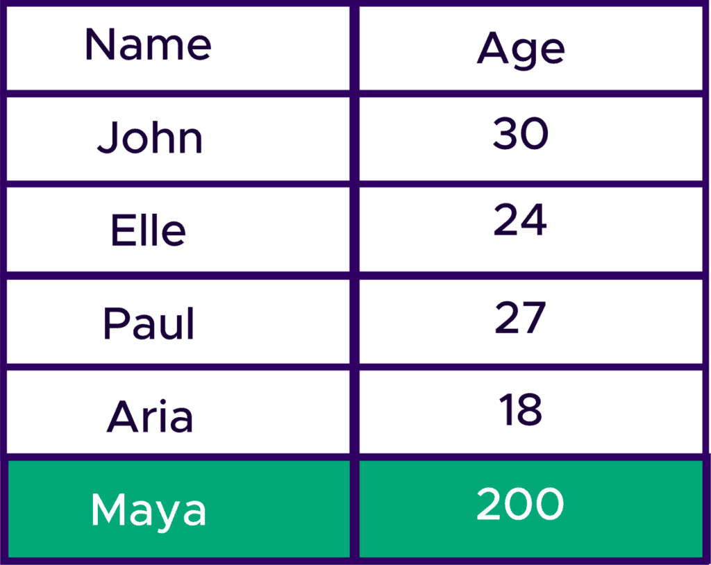
- Using tables: This is the simplest method, where tables and worksheets are eyeballed to detect these outliers. This technique is possible if the data sample is small, but the observation increases to the thousands and beyond, it becomes close to impossible. From the table below, it is evident that Maya stands out from the other instances.
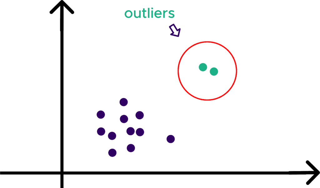
- Using graphs: This is one of the best ways to identify outliers in data. This technique makes use of visualizations like graphs and charts to see the difference that exists. Two plots that enable quick detection of these outliers graphically are scatter-plots and boxplots, respectively. The scatter plots depict the numeric data points on cartesian coordinates (typically for two variables).
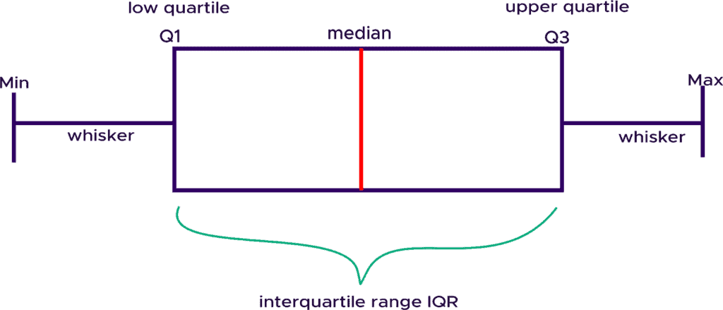
The boxplot, on the other hand, displays groups of numerical data points based on their quartiles. The box has whiskers extended which indicates variability outside the upper and lower quartiles.
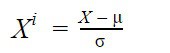
- Using statistical methods: This is a complex yet precise method that finds the statistical distribution that closely approximates the data distribution and uses statistical methods to detect the discrepant points. Two main techniques exist under this method, Z-score and IQR score, respectively. Z-scores measure the usualness of a data instance when the data follows a normal distribution. Z-scores find the relationship between the standard deviation of observation to the mean of the data. It can be seen as the number of the standard deviation of each data instance above and below the mean of the data. Values far from the mean are tread as outliers. On a scaled data, it is common practice to take values as outliers if their z-score value is outside the threshold of 3 and -3.
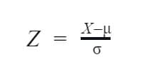
Where X is the observation
The IQR Score creates a fence outside the first quartile (Q1) and the third quartile(Q3) of the data. Any data point value that falls outside the fence is considered an outlier.
Fence lower range = Q1 – 1.5IQR
Fence upper range =Q3 + 1.5IQR
Note: IQR = Q3 -Q1
Data transformation: This is a preprocessing step that converts data from one format or structure to another to help find patterns or to improve the efficiency of the various data mining models. Most data mining algorithms require the data to be parsed in specific formats to work efficiently. Data transformation provides the original data with an alternative representation. Subtasks of data transformation are feature engineering, data aggregation (summarization), data normalization, discretization, and generalization. These subtasks will be independently segregated and exclusively explained. The transformation processes are known as data wrangling or data mugging. Most of these transformational processes can be simple or complex based on the required changes to transform and map data from one(source) format to another (target).
Data normalization: This is known as feature scaling. It is a data transformation step that expresses features in the same measurement units or a standard scale. Most of the time, data consists of features with varying magnitude, unit, and range. To normalize means to bring to a standard state by multiplying an attribute by a factor that yields the quantity to a desired range of values. Normalizing data attempts to give five independent features equal weights to prevent bias (variables dominating others) when building various data mining models.

Some data mining algorithms are sensitive to data normalization, while others are invariant to it.
- Gradient descent algorithms: Algorithms with gradient descent as optimization techniques (such as Neural Network, Linear Regression, and Logistic Regression) requires data to be scaled. Gradient descent is an iterative technique that minimizes a given function to its local minimum by measuring changes in all weights regarding the change in error. The difference in feature ranges will cause different steps for each feature, leading to an erratic descent towards the minima. To ensure a smooth gradient descent, it is required for the data to be scaled and updated at the same rate for all features and yield a quick convergence towards the minima.
- Distance-based algorithms: Algorithms that utilizing distance measures like hamming distance, Euclidean distance, Manhattan distance, and Minkowski distance (like K-Nearest Neighbors, Learning Vector Quantization (LVQ), Self-Organizing Map (SOM), K-Means Clustering) are more affected by the range of features. These algorithms use various distance functions to evaluate the distance between data points to determine their similarity. When features have different scales, a bias is introduced to the system as higher weightage is probably given to features with a higher magnitude. Therefore it is pertinent to scale data before employing a distance-based algorithm so that all the features contribute equally to the results.
- Tree-based algorithms: Algorithms constructed on branches and nodes entities (such as Decision Tree, Random Forest, and Boosting) recursively split training samples, using different features from a dataset at each node. The range of features has nothing to do with splitting, making tree-based algorithms insensitive to the varying scale of features.
Let explore the available methods for feature scaling. There are three main methods of scaling data.
- Normalization: This method is also known as Min-Max scaling. It transforms the numerical values of a feature by rescaling it to a given range.
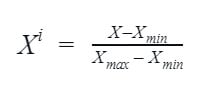
Where X is the given data instance;
Xmax is the feature maximum value
And Xmin is the feature minimum value
- Standardization: This is also known as the mean removal method. As the name implies, this method removes the mean values of the data from the data instance under consideration and scaling to unit variance.
- Robust Scaling: This method utilizes the interquartile range (IQR). This method eliminates the median from the data instance and scales the data between the first quartile (Q1) and third quartile (Q3), making it robust to outliers.
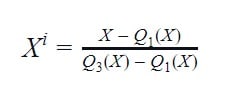
Where Q1 is the first quartile
Q3 is the third quartile
- Data Aggregation: This is a data transformation strategy that combines two or more attributes. This assemblage yields a summarized new data form that provides statistical analysis such as descriptive statistics like average, median, minimum, maximum, sum, count, standard deviation, variance, and mean absolute deviation. This summarized data may be gathered from multiple data sources with the intent of combination into a summary for data analysis. At times, information needs to be aggregated from an individual level to a focus level to get insights into the nature of a potentially large dataset.

Aggregation serves the following purposes:
- Reduces the variability (standard deviation) in the data and consequently reduces random noise in the data. It makes the data set more stable and easier to understand the granularity.
- Aggregation tends to provide a high-level view of the data as it changes scales. A good example is aggregating days to weeks, weeks to months.
- Aggregation facilitates faster processing time and reduces memory storage as it results in a smaller data set (data reduction).
- Data Discretization: Continuous data mathematically have an infinite degree of freedom. Often it is easier to understand continuous data when grouped into relevant categories. For example, taking height as a continuous variable, dividing it into three categories tall, short and average, is reasonable. Discretization is the process of converting continuous variables into a finite set of intervals. These contiguous intervals (bins) transcend the range of the continuous variable in scope and are treated as ordered and discrete values. Discretization is a data reduction method as it converts a large number of data values into small ones by grouping them into bins. Data discretization aids the maintainability of data. It also increases processing speed as memory space is traded off. One of the main challenges of discretization is choosing the optimal number of intervals(bins) and respective widths.
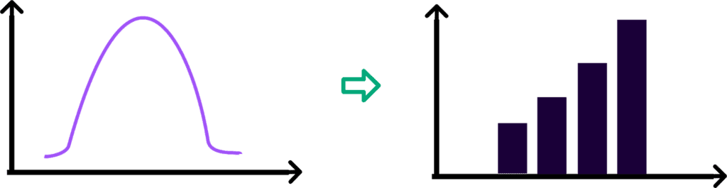
There are three types of discretization:
- Unsupervised discretization: In this type of discretization, the class label is not considered in transforming the continuous variable. This technique consists of the following methods:
- Equal-interval (equal-width) binning: split the whole range of numbers into intervals with equal size.
- Equal-frequency (equal-depth) binning: use intervals containing an equal number of values.
- Cluster analysis: Clustering algorithms may be implemented by partitioning the continuous variable values into clusters or classes to isolate a computational feature.
- Supervised discretization: This type of discretization divides the continuous variable in a fashion that provides maximum information about the class label. This technique consists of the following methods:
- Using class boundaries: This method involves sorting the values of the continuous variable and placing breakpoints between values belonging to different classes.
- Entropy-based discretization: This method approaches the iterative partitioning of a continuous attribute by bisecting the initial values so that the resulting interval gives the minimum entropy. The entropy can be calculated as follows:
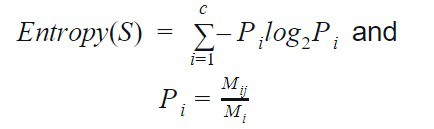
Where c is the number of the different class label
Pi is the probability of class j in the ith interval
Mi is the number of values in the ith interval of the partition
Mij is the number of values of class j in interval i
- Concept hierarchy generation: This is recursively applying partitioning and discretization methods. This involves mapping nominal data from low-level concepts to higher-level concepts. This method has two approaches:
- Top-down mapping: commence mapping from the top with general concepts and moves to the bottom to the specialized concepts.
- Bottom-up mapping: commence mapping from the bottom with specialized concepts and moves to the top to the generalized concepts.
- Attribute/feature construction: This is the construction of new attributes from the given set of data attributes and domain knowledge. It is comprehensively explained in a previous post on our blog here.
- Categorical encoding: Categorical data constitute discrete values that belong to a specific finite of classes. Category variables are expressed as text data and thus adds additional complexities in the semantics of each class. These complexities make it difficult for machine learning algorithms to work with categorical data compared to numerical data. Category encoding is a set of techniques employed to convert categorical variables into numerical representations. Categorical features are of two types:
- Ordinal: has an intrinsic order—for example, sizes (small, medium, and big).
- Non-ordinal: has no inherent order—for example, colors (red, blue, green).
The various encoding scheme applied to categorical data are as follows:
- Label Encoding: This is also known as Integer Encoding or Ordinal Encoding. This scheme is employed when the order is required to be preserved, making it a good fit for ordinal categorical data. It converts the respective labels into integer values between 0 and n-1, where n is the number of distinct classes in the categorical variable.
- One Hot Encoding: This is applied to categorical data with no intrinsic order; this scheme maps each level of a categorical feature to create a new variable known as indicator/dummy variable. The number of new dummy variables created depends on the levels present in the categorical feature. These dummy/indicator variables are a vector of binary elements 0s and 1s, where 0 and 1 signify the absence and presence of a given category. This method can cause memory inefficiency as it creates an enormous number of columns if the category level is significant.
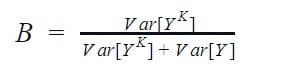
- Target Encoding: This technique uses Bayesian probability to utilize information from dependent(target) variables to encode categorical data. This scheme applies to both continuous and categorical targets. For continuous targets, the mean of the target variables for each category is calculated and used to replace the respective class. In the case where the target is a categorical variable, the categories are replaced with posterior probabilities of the target. Target encoding is prone to data leakage and overfitting but can be efficient when done correctly. Target encoding is built into famous boosting machine learning algorithms like Catboost and LightGBM.
- Hashing encoding: This technique is employed in high cardinality categorical data. It uses a hash function to map categorical data to fixed-size values. This scheme encodes the categorical variable into a sparse binary vector and has the option to control the resultant dimensional space by presetting the output dimension. This property of fixing the number of dimensions can be detrimental as it may lead to loss of information and collision (where the same hash value can represent multiple values).
- Binary Encoding: This encoding scheme is a mix of one-hot encoding and hash encoding. It creates fewer new features than the one-hot encoding scheme and yet preserves the uniqueness in the categorical data. It utilizes binary numbers as it transforms and stores the categorical values in binary bit strings. Each binary digit gets a column as a new feature in the data; if there are ‘n’ unique classes in the categorical variable, this encoding scheme outputs.
It works well with higher dimensionality categorical data but is prone to information loss and lacks human-readable sense.
- Weight-of-Evidence (WOE) Encoding: This encoding scheme is functional for encoding categories in the classification domain. WOE measures how much the hypothesis is supported or impaired by the evidence. This method was developed to create predictive models for churn rates in the financial industry as it evaluates risks (good/bad).
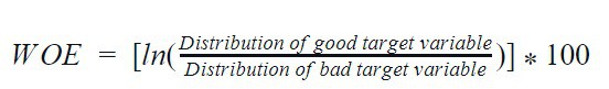
WOE = [ln(Distribution of good target variableDistribution of bad target variable)]*100
The WOE is greater than 0 if the target being good is more significant and less than 0 if the target being bad is more significant. Note here, good and bad are two classes used to explain the concept. WOE is best suited for logistic regression. It also creates a monotonic relationship between the dependent and independent variables but is susceptible to overfitting and loss of information.
- Frequency encoding: It is also known as Count encoding and as the name implies, each categorical is encoded with its respective observation percentage/count in the data. It simply uses the frequency of each category for numerical representation of each class. It aids proper weight assignment in cases where the categorical data is related to the target. It does not increase the data dimensions. It excels in tree-based algorithms but is not suitable for linear models. There can be a loss of information if we have an equal frequency distribution of classes as the encoding values will be the same value.
- Sum Encoding: This is also known as Deviation and Effect encoding. This encoding scheme is similar to One Hot Encoding except it represents the categorical data using three values i.e. 1,0, and -1. One of the categories is held at a constant value of -1 throughout all the dummy variables columns.
- Helmert Encoding: This is best suited for ordinal categorical values. In this encoding scheme, the mean of the dependent variable is juxtaposed to the mean of the dependent variable across all categorical levels. It can be done in two ways based on the comparison: forward (next levels) and reverse (previous levels). It is commonly used for regression tasks.
- James-Stein Encoding: This scheme is target-based and is inspired by the James–Stein estimator. The intuition behind this technique is to improve the estimation of the category’s mean target by using the formula:
The improvement is via shrinking the target mean towards a more central average, the hyperparameter ‘B’ accounts for it — the power of shrinking. This hyperparameter can be tuned via cross-validation and also has a formula:
- BaseN Encoding: This scheme encodes the categories based on predefined base-N representation. For example, base 1 corresponds to One-Hot encoding and base 2 is identical to a binary encoding. N represents the number of categories, so in a high cardinality situation, higher bases like 4 or 8 can be employed.
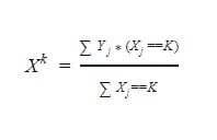
- Leave-one-out Encoding: This is another target-based encoder. It is similar to target encoding but when calculating the mean target for a category level the current row’s target is kept out. This can help reduce the effect of outliers. Leave-one-out Encoding: This is another target-based encoder. It is similar to target encoding but when calculating the mean target for a category level the current row’s target is kept out. This can help reduce the effect of outliers. This scheme calculates the mean target of category k for j observation if observation j is eliminated from the data as:
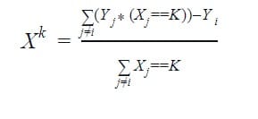
While the test set encoding is replaced with the mean target of the category k in the training dataset as:
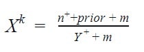
- M-Estimate Encoder: This is a simplified version of the Target encoder. It has a hyperparameter ‘m’ that aids stronger shrinking. The ideal range of m values is in the range of 1 to 100.
Data integration: This step involves the merging of multiple heterogeneous datasets into a coherent dataset. This unification of these disparate data sources is to reduce and avoid redundancies and inconsistencies in the data. This step also provides consistent access and delivery of unified data that cut across various subjects and structure types and meet its functional requirements. Aside from data enrichment, this step further increases the depths of business intelligence, data analytics, and information delivery.

Data Reduction: This is the process of decreasing the volume/size of the dataset without loss in originality. This reduction process yields a condensed representation of the dataset that maintains the structure and integrity of the original data. In dimensionality reduction, data encoding or data transformation techniques are employed to obtain a reduced or compressed form of the original data. At a glance, the downsizing of data might seem optional, but it is a pivotal step in building better models. Data mining algorithms have certain time complexity that is dependent on the size of the input. Also, data reduction aids the decrease of complexity in data and improves the quality of models yielded.
Let’s explain the various strategies that are employed to downsize data:
- Dimensionality reduction: This technique achieves data reduction by eliminating irrelevant or redundant features (or dimensions) while retaining some meaningful properties of the original data. Dimension reduction approaches are divided into feature selection and feature extraction.
- Feature selection: This is also known as the variable selection and attribute selection. It selects relevant features for model building. Feature selection reduces training session time and overfitting by enhancing generation. It prevents the curse of dimensionality and increases model interpretability. Feature selection aims to find the minimum set of attributes resulting in probability distribution closely identical to the original distribution with all attributes. Feature selection employs three strategies: filter strategy (e.g. information gain), the wrapper strategy (e.g.accuracy guided search), and the embedded strategy (selected features based on prediction errors).
- Feature Extraction: This initiates modification of the internal values representing the attributes, thus creating artificial substitute attributes and merging attributes. Feature Extraction aims to derive informative and non-redundant features from the dataset that subsequently leads to faster and better models. It is mainly applied in image processing to isolate sections of an image or video.
The various methods used for dimensionality reduction include:
- Principal Component Analysis (PCA)
- Linear Discriminant Analysis (LDA)
- Generalized Discriminant Analysis (GDA)
- Numerosity Reduction: This technique reduces the data volume by replacing the original data with an alternative smaller data representation. This technique can either be parametric or non-parametric.
- Parametric methods: This method uses the data parameters to represent the entire data by fitting the original data to a model that adequately estimates the data. Regression and Log-Linear methods can be used to achieve parametric reduction.
- Non-parametric methods: This method doesn’t employ models to represent the data but rather data distribution, frequency, and distance measures. Histogram, clustering, and sampling can be used to achieve non-parametric reduction.
Data Preprocessing tools
Data science is rapidly evolving and there are many tools to assist in data-driven processes. In order to be stern in scope, data preprocess can be done in any tool that aids data manipulation. Some of the top tools as of the time of writing this articles includes:
- Python
- Javascript
- R
- Excel
- SAS
- Weka
- Apache Spark
- Power BI
- Tableau
The hands-on section in this article was covered using Python because of extensive and easily accessible libraries for data analysis.
Hands-on section of data preprocessing
n the previous section the various preprocessing tools were highlighted, Python is used to explain how data preprocessing can be carried out. Python is used because of its simplicity and readability, so beginners can understand the various concepts and focus less on the programming syntax. Also, Python is an exhaustive open source library that covers data analysis, data visualization, statistics, machine learning and deep learning.
Case study: Titanic datasets. Goal: Predict the survivors. To read more about the titanic dataset, click here. The famous titanic dataset will be used to explain the various concepts.
In order to carry out data science operations such as data cleaning, data aggregation, data transformation, data visualization and other insight generation operations we need the dataset to be investigated and analyzed to be read into python and the various libraries to aid data preprocessing.
Formats of data commonly encountered in data science projects
- CSV
- XLSX
- TXT
- JSON
- XML
- ZIP
- HTML
- DOCX
- MP3
- MP4
- SQL
- Images
- Hierarchical data format
					### Importing relevant libraries
import numpy as np
import pandas as pd
import matplotlib.pyplot as plt
import seaborn as sns

### Reading the dataset
train_df = pd.read_csv('../data/train.csv')
test_df = pd.read_csv('../data/test.csv')
- Numpy: to perform a number of mathematical operations on arrays.
- Pandas: to handle data manipulation and wrangling.
- Matplotlib & Seaborn: to aid visualization of data.
### Getting overview of the datasets
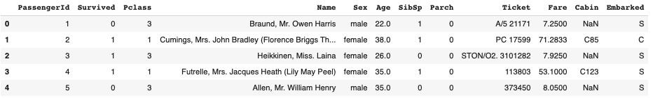
train_df.head()
test_df.head()
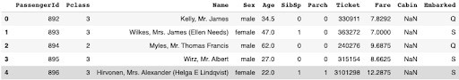
It can be observed that the test set has the same features of the training set except the Survived feature. The Survived feature is the target variable.
A brief description of the data generated from the metadata is as follows:
- Survived
- 0: No
- 1:
- pclass: Ticket class-A proxy for socio-economic status
- 1: Upper
- 2: Middle
- 3: Lower
- Age: Numerical value of age
- SibSp: Number of siblings or Spouses aboard the titanic
- Parch: Number of parents or Children aboard the titanic
- Ticket: Ticket number
- Cabin: Cabin number
- Embarked:Port of Embarkation
- C: Cherbourg
- Q: Queenstown
- S: Southampton
Variable notes:
- age: Age is fractional if less than 1. If the age is estimated, is it in the form of xx.
- sibsp: The dataset defines family relations in this way
- Sibling = brother, sister, step-brother, step-sister
- Spouse = husband, wife (mistresses and fiancés were ignored)
- parch: The dataset defines family relations in this way
- Parent = mother, father
- Child = daughter, son, stepdaughter, stepson
- Some children travelled only with a nanny, therefore parch=0 for them.
#Split the dataset into independent and dependent
target = train_df['Survived']
train_df.drop(columns='Survived', inplace=True)
#have a preview of the descriptive statistics
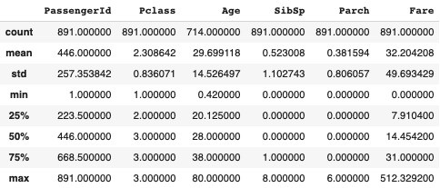
train_df.describe()
test_df.describe()
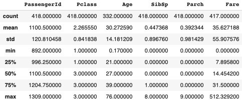
The descriptive statistics summarizes the data. It outputs the number of instances(counts), mean value of each numerical variable as well as standard deviation, minimum value, maximum value, the first quartile (25%), second quartile (50% also the median) and third quartile (75%).
Next, check the formats of the various columns(features):
In Pandas, we use:
- .dtype() to check the data type
.astype() to change the data type
train_df.dtypes
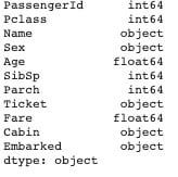
test_df.dtypes
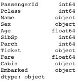
The various data types are in order. Int, float, object represent Integer, decimal numbers and categorical values respectively.
Check for missing values
Evaluating for Missing Data
The missing values are converted to Python’s default. We use Python’s built-in functions to identify these missing values. There are two methods to detect missing data:
- .isnull()
- .notnull()
The output is a boolean value indicating whether the value that is passed into the argument is in fact missing data.
Check for missing values: The missing values are converted to Python’s default. We use Python’s built-in functions to identify these missing values. There are two methods to detect missing data:
- .isnull()
- .notnull()
The output is a boolean value indicating whether the value that is passed into the argument is in fact missing data.
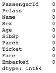
train_df.isnull().sum()
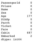
test_df.isnull().sum()
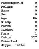
The cabin feature has a significant amount of instances missing, hence the feature will be dropped.
					#dropping the cabin feature
train_df.drop(columns='Cabin', inplace=True)
test_df.drop(columns='Cabin', inplace=True)
					# To replace the missing values in 'Age' with a value of central tendency, lets see the distribution
train_df['Age'].hist();
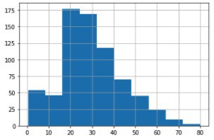
					age_mean_val1 = train_df['Age'].mean()
age_mean_val2 = test_df['Age'].mean()

train_df['Age'].replace(np.nan, age_mean_val1, inplace=True)
test_df['Age'].replace(np.nan, age_mean_val2, inplace=True)
					### Handling the missing values in the 'Embarked' features in the training set

# Since its categorical, we can use the mode (highest occurence to replace the missing values)
train_df['Embarked'].value_counts()
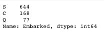
					# Replacing the missing values in the 'Embarked' features with 'S'
train_df['Embarked'].replace(np.nan, 'S', inplace=True)
					### handling the missing values in the 'Fare' feature in the test set, lets see the distribution
test_df['Fare'].hist()
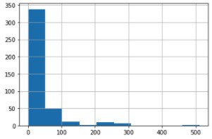
					# Due to the skewness, replace missing values with the median

fare_median_val = test_df['Fare'].median()
test_df['Fare'].replace(np.nan, fare_median_val, inplace=True)
					#Cross checking the missing values below:
train_df.isnull().sum()
test_df.isnull().sum()
Dropping irrelevant features
Since our goal for insights generation majorly is Machine Learning, which entails pattern recognition in the datasets and predictions, so features are too unique that they are irrelevant such as
- PassengerId
- Name* (But we can extract some things from this as we will see in a later section. So, we won’t drop it now)
- Ticket
					cols_to_drop = ['PassengerId','Ticket']
train_df.drop(columns=cols_to_drop, inplace=True)
test_df.drop(columns=cols_to_drop, inplace=True)
Handling Categorical features: Categorical features are features which can take on values from a limited set of values
Machine learning models cannot work with categorical features the way they are. These features must be converted to numerical forms before they can be used. The process of converting the categorical features to numerical features is called encoding.
There are numerous types of encoding available, and the choice of which to use depends on the categorical type. So first, let’s understand the different categorical types there are.
The various encoding schemes were discussed earlier. To perform automated encoding, we will use an efficient library called categorical_encoders. This library offers numerous encoding schemes out of the box and has first hand support for Pandas DataFrame.
To install the library, you can use pip as follow:
!pip install category_encoders
					### Review data types
train_df.info()
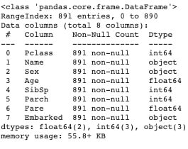
It can be observed that..
- Name: Non ordinal(unique)
- Sex: Non ordinal
- Embarked: Non ordinal
So, a preferred encoding scheme would be one-hot encoding.
import category_encoders as ce

cats = ['Sex', 'Embarked']
one_hot_enc = ce.OneHotEncoder(cols=cats)

#The various encoding scheme discussed previously can be initiated as
# encoder = ce.BaseNEncoder(cols=[...])
# encoder = ce.BinaryEncoder(cols=[...])
# encoder = ce.CountEncoder(cols=[...])
# encoder = ce.HashingEncoder(cols=[...])
# encoder = ce.HelmertEncoder(cols=[...])
# encoder = ce.JamesSteinEncoder(cols=[...])
# encoder = ce.LeaveOneOutEncoder(cols=[...])
# encoder = ce.MEstimateEncoder(cols=[...])
# encoder = ce.OneHotEncoder(cols=[...])
# encoder = ce.OrdinalEncoder(cols=[...])
# encoder = ce.SumEncoder(cols=[...])
# encoder = ce.TargetEncoder(cols=[...])
# encoder = ce.WOEEncoder(cols=[...])
### Fitting and transforming the datasets
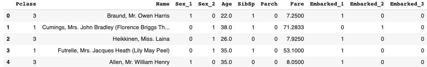
train_df = one_hot_enc.fit_transform(train_df)
test_df = one_hot_enc.transform(test_df)
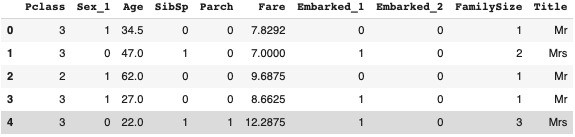
train_df.head()

test_df.head()
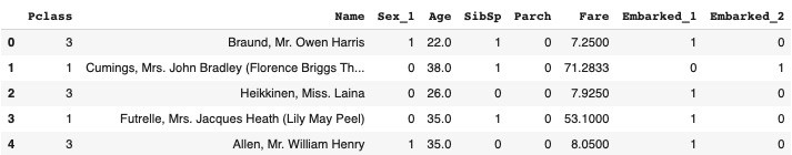
					# To avoid dummy trap, you have to drop one of the generated encoded class for parent feature
train_df.drop(columns=['Sex_2','Embarked_3'], inplace=True)
test_df.drop(columns=['Sex_2','Embarked_3'], inplace=True)
train_df.head()

Feature engineering is the process of using domain knowledge to extract features from raw data via data mining techniques. These features can be used to improve the performance of machine learning algorithms.
					# Creating FamilySize feature
train_df['FamilySize'] = train_df['SibSp'] + train_df['Parch'] + 1
test_df['FamilySize'] = test_df['SibSp'] + test_df['Parch'] + 1

# Using Regular Expression (More information on regular expression is the bonus section)
#Extract title from name of the passenger
train_df['Title'] = train_df.Name.str.extract(' ([A-Za-z]+)\.', expand=False)
train_df = train_df.drop(columns='Name')

test_df['Title'] = test_df.Name.str.extract(' ([A-Za-z]+)\.', expand=False)
test_df = test_df.drop(columns='Name')
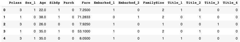
train_df.head()
test_df.head()
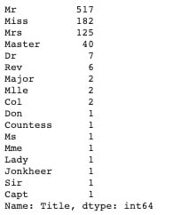
train_df.Title.value_counts()

					# Categorizing the titles
train_df['Title'] = train_df['Title'].replace(['Dr', 'Rev', 'Col', 'Major', 'Countess', 'Sir', 'Jonkheer', 'Lady', 'Capt', 'Don'], 'Others')
train_df['Title'] = train_df['Title'].replace('Ms', 'Miss')
train_df['Title'] = train_df['Title'].replace('Mme', 'Mrs')
train_df['Title'] = train_df['Title'].replace('Mlle', 'Miss')

test_df['Title'] = test_df['Title'].replace(['Dr', 'Rev', 'Col', 'Major', 'Countess', 'Sir', 'Jonkheer', 'Lady', 'Capt', 'Don'], 'Others')
test_df['Title'] = test_df['Title'].replace('Ms', 'Miss')
test_df['Title'] = test_df['Title'].replace('Mme', 'Mrs')
test_df['Title'] = test_df['Title'].replace('Mlle', 'Miss')
train_df.Title.value_counts()
test_df.head()
NOTE: The Title column is still a categorical feature which is not ordinal, so we ought to encode it.
					cats = ['Title']
one_hot_enc = ce.OneHotEncoder(cols=cats)

### Fitting and transforming the datasets
train_df = one_hot_enc.fit_transform(train_df)
test_df = one_hot_enc.transform(test_df)
train_df.head()
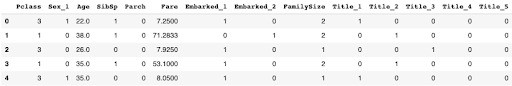
					# To avoid dummy trap
train_df.drop(columns=['Title_5'], inplace=True)
test_df.drop(columns=['Title_5'], inplace=True)
train_df.head()
Feature Scaling is a technique to standardize the independent features(what we are using to predict) present in the data in a fixed range. If feature scaling is not done, then a machine learning algorithm tends to weigh greater values, higher and consider smaller values as the lower values, regardless of the unit of the values.
The various techniques were explained earlier and sklearn library provides access to their functionality
					#Save the header
header = train_df.columns.to_list()
					#Install sklearn if it is your first time using it

#!pip install scikit-learn

#Lets normalize
from sklearn.preprocessing import MinMaxScaler

#In the case of Standardization
#from sklearn.preprocessing import StandardScalar

#In the case of Robust Scaling
#from sklearn.preprocessing import RobustScaler

#Instantiating the object
norm = MinMaxScaler()

#Fitting and transforming the dataset
train_df = norm.fit_transform(train_df)
test_df = norm.transform(test_df)
Best practice of data preprocessing
- Getting metadata will enable you to get underlying definitions or descriptions of the data.
- Defining the project goals will guide you towards the desired expectation.
- Establishing quality key performance indicators (KPIs) for data will steer in the respective data preprocessing technique to use.
- Develop a workflow: Data preprocessing steps are not stern and defined; you can classify your workflow into independent blocks, each with particular functionality.
- Research on new techniques and approaches, the data science space is fast-paced and full of innovation. Also, be on the look for new and better ways of performing various tasks.