Table of Contents
Classifying sentences is a common task in the current digital age. Sentence classification is being applied in numerous spaces such as detecting spam in emails, determining the sentiment of a review, and auto-tagging customer queries just to mention a few. These applications have been enabled by recent advancements in machine learning and deep learning. The availability of computation power and large datasets has also enabled the training of highly performant deep learning models. Machine learning frameworks such as Scikit-learn and deep learning frameworks such as TensorFlow and PyTorch have also played a huge role in advancing the natural language processing space.
This article will explore how to classify sentences using various tools such as Scikit-learn, TensorFlow, and PyTorch. Once you are done you will be able to:
- Obtain a text data set
- Clean the dataset
- Perform text related preprocessing
- Build a machine learning and deep learning model for text classification
- Evaluate the text classification model
Let’s get started.
A primer on (Deep) Neural Networks
Artificial neural networks are built to mimic the working of the human brain. As you can see from the image below, the dendrites of the human brain represent the input in the artificial neural network. The axion terminals then represent the output of the neural network. The image on the right represents a network with only one hidden layer. A network containing several hidden layers is referred to as a deep neural network.
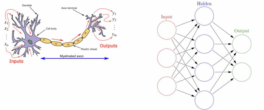
Image source. Brain neuron the left. Simple neural network on the right.
You may now be wondering how exactly neural networks work. Let’s look at this next.
How do Neural Networks work?
Neural networks work by performing some computations on the given data and then emitting an output. The process looks like this:
- Weights and biases are initialized to small numbers close to zeros. There are several ways of initializing them, for instance, using a normal or uniform distribution.
- The observations are then fed to the input layer.
- These observations are then propagated through the network and predictions are obtained. This is known as forward propagation. As the data passes through the hidden layers, an activation function is applied. A common one in these layers is the ReLu activation function. It caps all numbers to 0 and above.
- Before obtaining the final output `y` the result is passed through another activation function in the output layer. The activation function ensures that the network outputs the expected result. For example, in a classification problem, you want the final output of your model to be the probability of the input belonging to a certain class. Some common activation functions include the sigmoid that is used for binary classifications and the softmax that is used for multiclass problems where the labels are mutually exclusive.
- The next step is to compare the predicted result to the true results. The difference between the two is the error. The network will learn by adjusting the weights based on the error. This is done using a loss function, also known as a cost function. The goal is to minimize this cost function. The choice of a cost function will depend on the problem, for instance, you will use classification loss functions for classification problems.
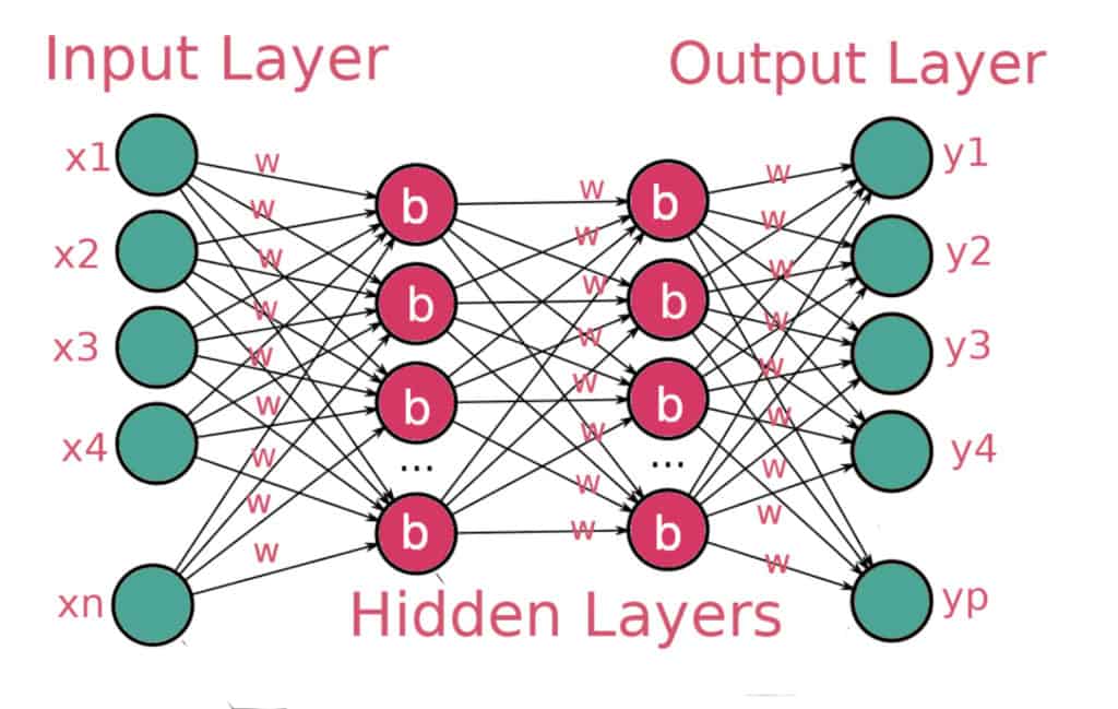
Image source. An example of a deep neural network.
- The next step is to propagate these errors back to the network so that it can adjust the weights. This is how the network learns. This is known as backpropagation. It is done via gradient descent. Gradient descent is an optimization strategy that aims at obtaining the point with the least error. There are several variants of gradient descent. The common ones include Batch gradient descent, Stochastic gradient descent, and Mini-batch gradient descent. Batch gradient descent uses the entire dataset to compute the gradient of the cost function. It is usually slow because you have to compute the gradient of the entire dataset before making a single update. In Stochastic gradient descent, the gradient of the cost function is computed from one training example in every iteration. As a result, it is faster than batch gradient descent. Mini-batch gradient descent uses a sample of the training data to compute the gradient of the cost function.
Convolutional Neural Networks are also artificial neural networks. With that intuitive understanding of neural networks, let’s dive straight into Convolutional Neural Networks.
What are Convolutional Neural Networks?
Convolution Neural Networks(CNNs) are multi-layered artificial neural networks with the ability to detect complex features in data, for instance, extracting features in image and text data. CNNs have majorly been used in computer vision tasks such as image classification, object detection, and image segmentation. However, recently CNNs have been applied to text problems.
The general architecture of a Convolutional Neural Network
A Convolutional Neural Network is made up of two main layers:
- A convolution layer for obtaining features from the data
- A pooling layer for reducing the size of the feature map
How does the CNN architecture work?
The convolution layer and pooling layers are the main building blocks of a convolutional neural network. Let’s now take a look at the operations that happen in those layers.
What is Convolution?
Convolution is the process through which features are obtained. These features are then fed to the CNN. The convolution operation is responsible for detecting the most important features. The output of the convolution operation is known as a feature map, a convolved feature, or an activation map. The feature map is computed through the application of a feature detector to the input data. In some deep learning frameworks, the feature detector is also referred to as a kernel or a filter. For instance, this filter can be a 3 by 3 matrix. You are free to choose any filter that works well for your problem.
The feature map is computed through an element-wise multiplication of the kernel and the matrix representation of the input data. This ensures that the feature map passed to the CNN is smaller but contains all the important features. The filter does this by sliding step by step through every element in the input data. These steps are known as strides and can be defined while creating the CNN.
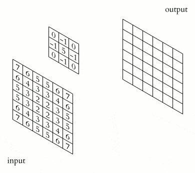
Source. The convolution operation
Channels
Image data usually has three channels ie red, green, and blue. Convolutions are usually applied across the channels. Different filters can be applied to every channel and later merged into a single vector. In the text processing realm, channels can be thought of as the sequence of words, word embeddings, and the shape of the words. The different kernels applied to the words can then be merged into a single vector.
Pooling
Pooling works by placing a matrix, say a 2 by 2 matrix, on the feature map and performing a certain operation. For instance, in max-pooling, the maximum number falling within that matrix is picked. In average pooling, the average of the numbers falling within that matrix is computed. In min pooling, the minimum number falling in that matrix is used. The result is known as a pooled feature map. Pooling ensures that the network can detect features irrespective of their location. Pooling also ensures that the size of the data passed to the CNN is reduced further.
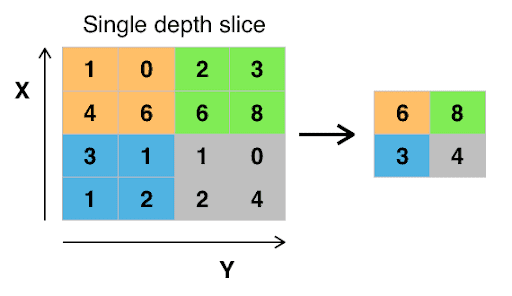
Source. Pooling operation
Flattening
Flattening involves converting the pooled feature map into a single column that will be passed to the fully connected layer.
Fully connected
The flattened feature map becomes the input of the neural network. This is then passed to a fully connected layer. Before the final output is obtained, the result is passed to an appropriate activation function. For instance, the sigmoid activation function in the case of binary problems and softmax in the case of multi-class problems.
CNN hyperparameters
When building Convolution Neural Networks, deep learning frameworks will usually allow you to tune some of the items discussed above. These include:
- The kernel size
- The number of filters
- The height and width of the strides
- The activation function to be used
- How the kernel should be initialized
- The way the bias will be initialized
You have covered a lot of ground this far. Armed with this information let’s now define a baseline model for a text classification problem.
Defining a baseline model
A baseline model is a simple machine learning model that can later be compared with more advanced models such as deep learning models. Ideally, the deep learning models should perform better than the baseline model. Let’s start by creating the baseline model.
Obtaining the dataset
The UCI Machine Learning portal provides numerous datasets for machine learning problems. Let’s download the Yelp reviews dataset for this illustration.
					!wget --no-check-certificate \
    https://archive.ics.uci.edu/ml/machine-learning-databases/00331/sentiment%20labelled%20sentences.zip \
    -O sentences.zip
The next step is to unzip the data.
					import os
import zipfile
with zipfile.ZipFile('sentences.zip', 'r') as zip_ref:
    zip_ref.extractall('sentences')
After that, the data can be loaded with a couple of parameters:
- `names` to give the data column headers since it doesn’t have any.
- `delimeter` to indicate that it’s tab-separated.
- `engine` to define the parsing engine as Python.
- `quoting` to determine the quoting behavior.
					import pandas as pd
df = pd.read_csv('sentences/sentiment labelled sentences/yelp_labelled.txt', delimiter = '\t', engine='python', quoting = 3,names=['review','status'])
Cleaning the dataset
Let’s now use the `re` module to clean this dataset. The objective here is to remove everything from the reviews but letters. This will involve removing all punctuation marks such as commas, question marks, etc. The `sub` function from the `re` module can be used to replace the punctuation marks. After removing the punctuation marks, convert all the reviews to lower case.
					import re
def clean_data(review):
    review = re.sub('[^a-zA-Z]', ' ',review)
    review = review.lower()
    return review
Let’s now apply this function to the reviews.
df['review'] = df['review'].apply(clean_data)
Removing stop words
The reviews also contain common words such as ‘the’, ‘at’, etc that don’t tell us much about the polarity of a sentence. Let’s get rid of those. To remove them, you have to employ the service of the Natural Language Toolkit (nltk). Let’s import the package and download the stop words.
					import nltk
nltk.download('stopwords')
The next step is to define the function that will remove all the common words from the reviews.
					def remove_stop_words(review):
    review_minus_sw = []
    stop_words = stopwords.words('english')
    review = review.split()
    review = [review_minus_sw.append(word) for word in review if word not in stop_words]
    review = ' '.join(review_minus_sw)
    return review
With the function in place, apply it to the reviews.

df['review'] = df['review'].apply(remove_stop_words)
Stemming
The next cleaning item on the menu is to convert the words in the reviews to their root form. For example, the word hated will be converted to its root form which is hate. This process is important because it reduces the number of words that will be fed to the machine learning model. `nltk` can assist us in converting the words in their root form. This can be done using the `WordNetLemmatizer` utility. This can also be done using the `PorterStemmer`.
What is the difference between Stemmers and Lemmatizers?
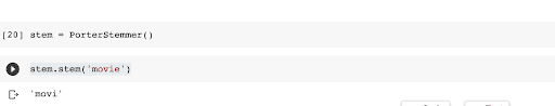
Stemmers use algorithms to remove suffixes and prefixes from words and the final words may not be the dictionary representation of a word. For instance, applying the `PorterStemmer` to the word movie results in `movi` which is not an actual word in the dictionary.
However, lemmatizers will usually convert a word to the dictionary representation. For example, the word `dogs` is converted to its root form which is `dog`.
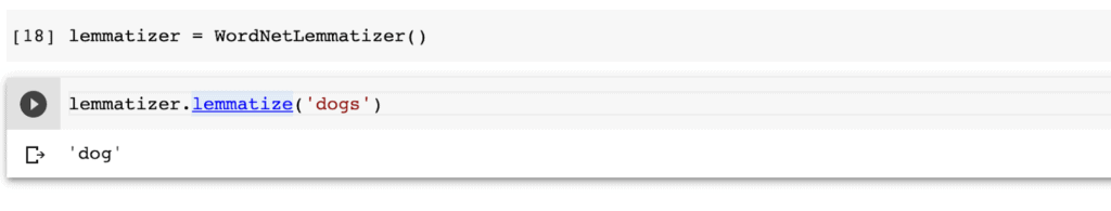
Let’s apply the `WordNetLemmatizer` here. The first step is to create the function that will be used to do this.
					nltk.download('wordnet')
#WordNet is a lexical database of English.
#Using synsets, helps find conceptual relationships between words
# such as hypernyms, hyponyms, synonyms, antonyms etc.
from nltk.corpus import stopwords
from nltk.stem import WordNetLemmatizer

def lematize(review):
    review = review.split()
    review = [lemmatizer.lemmatize(w) for w in review]
    review = ' '.join(review)
    return review
The next step is to apply the function to all the reviews.
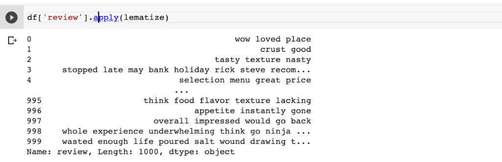
df['review'] = df['review'].apply(lematize)
Creating a bag of words model
As of this moment, the reviews are still in text form. However, they have to be converted into some numeric representation before they can be passed to the machine learning model. A common way for representing the reviews is through the bag of words model. This is how the bag of words model is created:
- Group all the reviews into a corpus. A corpus simply means a collection of many documents in this case the reviews.
- Take all the words in the corpus and create a column with each word.
- Represent each review with a row.
- If a certain word exists in the review, represent it by a 1, and if the word doesn’t exist in the review, represent it with a 0.
In the above representation, each word represents a single feature. The above process will result in a sparse matrix, i.e a matrix with a lot of zeros.
Let’s get the ball rolling by creating the corpus.
corpus = list(df['review'])
The numerical representation mentioned above can be obtained using the `CountVectorizer` from Scikit-learn. The function requires us to define the maximum number of words that will be used in the bag of words. The next step is to fit the instantiated `CountVectorizer` to the reviews.
					from sklearn.feature_extraction.text import CountVectorizer
cv = CountVectorizer(max_features = 1000)
 # Stop words are common words in English that don't tell us anything about the polarity of a review.
    # Such words include the, that, and a
# Converts a collection of text documents to a matrix of token counts
# max_features = maximum number of words we'd like to have in our bag of words model
X = cv.fit_transform(corpus).toarray()
y = df['status'].values
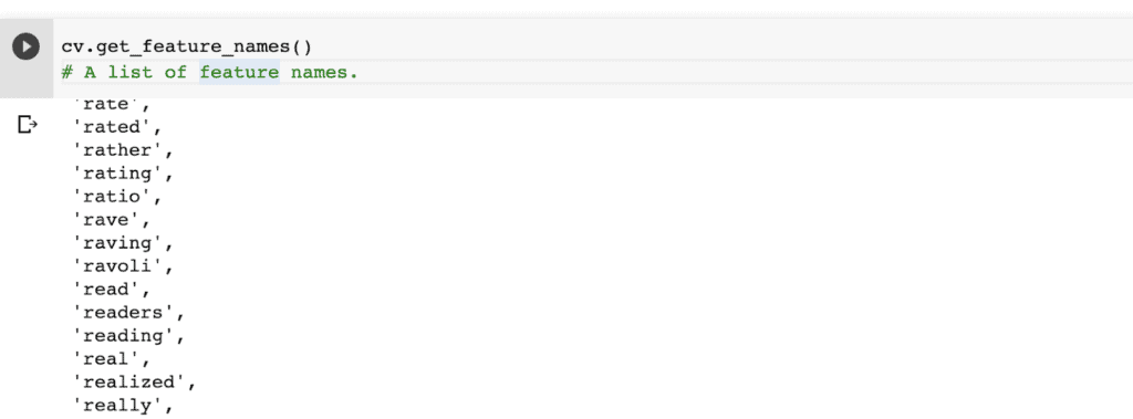
You can obtain a list of all features using the `get_feature_names` function.
cv.get_feature_names()
Here’s how the dataset looks after representing it using a Pandas DataFrame. Each column represents a word and each row is a review. The zeros and ones indicate whether a certain word exists in a review.
From occurrences to frequencies
In the above representation, the occurrence of words is being used to represent the bag of words model. This way of representing words has one major shortcoming. That problem is that longer documents (read reviews) will have a higher average count for a certain word than shorter documents. This challenge is addressed by dividing the total occurrences of a word by the total number of words. This results in new features known as tf, short for Term Frequencies. The problem with this is that common words will tend to have a higher tf. This challenge is addressed by downscaling the weight carried by the common words. The downscaling is referred to as tf–idf short for Term Frequency Inverse Document Frequency.
Consider a document containing 200 words, where the word love appears 5 times. The tf for love is then (5 / 200) = 0.025. Assuming there are one million documents and the word love occurs in one thousand of these, the inverse document frequency (i.e idf) is calculated as log(1000000 / 1000) = 3. The tf-idf weight is the product of these quantities i.e 0.025 * 3 = 0.075.
What has been described above can be implemented using the TfidfTransformer from Scikit-learn. Let’s import it and apply it to the reviews.
					from sklearn.feature_extraction.text import TfidfTransformer
tf_transformer = TfidfTransformer()
X = tf_transformer.fit_transform(X).toarray()
Fitting CountVectorizer followed by TfidfTransformer
Fitting the `CountVectorizer` followed by `TfidfTransformer` is so common that Scikit-learn has provided a function that can be used to apply both of them at the same time. That function is the `TfidfVectorizer`. Let’s apply it to the corpus.
					from sklearn.feature_extraction.text import TfidfVectorizer
tfidfVectorizer = TfidfVectorizer(max_features =1000)
X = tfidfVectorizer.fit_transform(corpus).toarray()
Searching for the best model
Now that the data is in the right form, split it into a training and validation set. Let’s use 20% for testing and the rest for training. For reproducibility, a random seed is also declared.
					from sklearn.model_selection import train_test_split
X_train_s, X_test_s , y_train_s, y_test_s = train_test_split(X, y , test_size = 0.20, random_state=101)
Fit several machine learning models and check which one results in the highest accuracy. The first step is to import these algorithms.
					from sklearn.ensemble import GradientBoostingClassifier
from sklearn.naive_bayes import GaussianNB
# Naive Bayes is a statistical classification technique based on Bayes Theorem
# common classifier used in sentiment analysis is the Naive Bayes Classifier.
from sklearn.experimental import enable_hist_gradient_boosting
from sklearn.ensemble import HistGradientBoostingClassifier # this is experimental
from sklearn.ensemble import RandomForestClassifier
from sklearn.linear_model import LogisticRegression
from xgboost import XGBClassifier
from lightgbm import LGBMClassifier
from catboost import CatBoostClassifier
classifiers = [GradientBoostingClassifier(),GaussianNB(),HistGradientBoostingClassifier(),
               RandomForestClassifier(),LogisticRegression(),XGBClassifier(),LGBMClassifier(),
               CatBoostClassifier(verbose=0)]
The next step is to fit all of them to the training set and check the performance on the testing set.
					from sklearn.metrics import confusion_matrix, classification_report,accuracy_score
for classifier in classifiers:
    classifier.fit(X_train_s,y_train_s)
    print(f'The {classifier}  Accuracy  is {accuracy_score(y_test_s,classifier.predict(X_test_s)) }' )
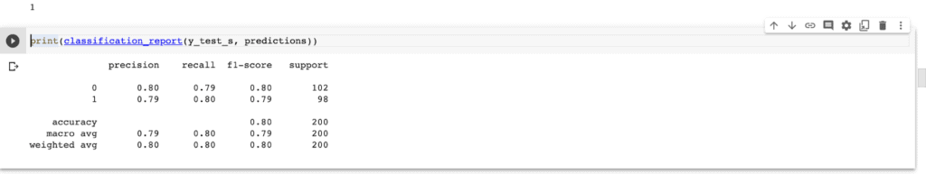
The logistic regression model has the highest accuracy.

Let’s use that model as our baseline model.
					classifier = LogisticRegression()
classifier.fit(X_train_s,y_train_s)
predictions = classifier.predict(X_test_s)
confusion_matrix(y_test_s, predictions)
Let’s now look at how this baseline model compares to an implementation using convolutional neural networks.
Understanding Convolutional Neural Networks for NLP
Convolutional Neural Networks have been widely applied in the computer vision realm. In this section, let’s take a look at how they can be applied to text data. Specifically, let’s use TensorFlow to build the convolutional neural network for text classification. However, before we get to the CNN, let’s look at how we can pre-process the data using TensorFlow.
Data preprocessing
Let’s start by splitting the data into a training and validation set.
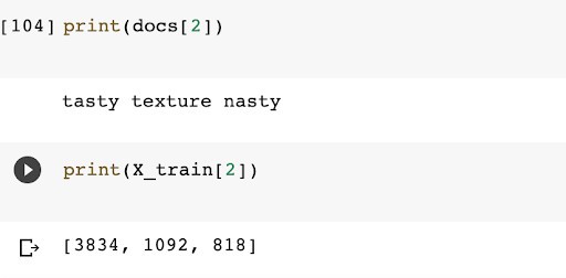
					docs = df['review']
labels = df['status']
from sklearn.model_selection import train_test_split
X_train, X_test , y_train, y_test = train_test_split(docs, labels , test_size = 0.20)
As seen earlier, the data has to be converted in some numerical representation. The `one_hot` function can be used to do this. The function will encode the reviews into a list of integers. It expects the following arguments:
- `text` that is the text to be encoded
- `n` the size of the vocabulary
- `filters` specify the characters to be removed from the reviews such as punctuation marks and any other special characters
- `lower` indicates if the reviews should be converted to lower case or not
- `split` dictates how the reviews should be split
from tensorflow.keras.preprocessing.text import one_hot

vocab_size = 5000

X_train = [one_hot(d, vocab_size,filters='!"#$%&()*+,-./:;<=>?@[\]^_`{|}~',lower=True, split=' ') for d in X_train]
X_test = [one_hot(d, vocab_size,filters='!"#$%&()*+,-./:;<=>?@[\]^_`{|}~',lower=True, split=' ') for d in X_test]
Here is how one review looks after the conversion.
Pad the sequences
At the moment each review is represented by a sequence of integers. The only problem here is that the sequences are of different lengths. Usually, the data passed to a machine learning model is of the same length. Therefore, the sequences have to be forced to be of the same length. This is done by padding shorter sequences with zeros and dropping off some integers on very long sequences. This means that you have to define the maximum length of every sequence. Let’s use 100 here. This is a number that can be modified until you obtain the optimal one for the problem in question.
					from tensorflow.keras.preprocessing.sequence import pad_sequences

max_length = 100
X_train = pad_sequences(X_train, maxlen=max_length, padding='post')
X_test = pad_sequences(X_test, maxlen=max_length, padding='post')
The dataset is now ready, let’s move on to creating the convolution neural network.
1-D Convolutions over text
The application of convolutional neural networks is the same as in image data. The only difference is that 1D convolutions are applied instead of 2D convolutions. In images, the kernel slides in 2D but in sequence data like text data the kernel slides in one dimension.
Let’s now take a look at how this CNN can be built.
1-D Convolutions over text
The convolution network will be made of of the following:
- An embedding layer that turns the data into dense vectors of fixed size. More on this later.
- A `Conv1D` with 128 units with the `relu` activation function.
- A `GlobalMaxPooling1D` layer that downsamples the input by taking the maximum value.
- A `Dense` layer with 10 units for the fully connected layer.
- An output layer with the sigmoid activation function because this is a binary problem.
from tensorflow.keras.layers import Dense, Embedding,GlobalMaxPooling1D
from tensorflow.keras.models import Sequential
from tensorflow.keras.layers import Dense
from tensorflow.keras.layers import Embedding

model = Sequential([
    Embedding(vocab_size, 8, input_length=max_length),
   Conv1D(128, 5, activation='relu'),
    GlobalMaxPooling1D(),
  Dense(10, activation='relu'),
  Dense(1, activation='sigmoid')
])
The next step is to prepare the model for training. Let’s apply the common `Adam` optimizer and the `binary_crossentropy` loss function.
model.compile(optimizer='adam', loss='binary_crossentropy', metrics=['acc'])
The next move is to train the model on the training set. You can also set the validation set at this stage.
history = model.fit(X_train, y_train, epochs=20, validation_data=(X_test, y_test))
Once, the training is done, the next step is to evaluate the model on the testing set.
					loss, accuracy = model.evaluate(X_test,y_test)
print('Testing Accuracy is {} '.format(accuracy*100))

The model achieves an accuracy of 74% which is lower than the baseline accuracy of 78%. You might get different results here because of the way weights are initialized. However, let’s look at whether this accuracy can be increased by using pre-trained word embeddings.
Convolutional Neural Networks applied to NLP
Pre-trained word embeddings can help in increasing the accuracy of text classification models. You can always train custom word embeddings just like we have done above. However, using pre-trained word embeddings is advantageous because they have been trained on millions of words. Obtaining such a dataset would be a challenge. Furthermore, training using such a massive dataset requires a lot of computation power.
What is a word embedding?
Data preparation
Let’s now create another sentence convolutional neural network to illustrate how to use pre-trained word embeddings. Before building the network, let’s showcase another way of preparing the text data for deep learning models. The first move is to split the data into a training and testing set.
					X = df['review']
y = df['status']
from sklearn.model_selection import train_test_split
X_train, X_test , y_train, y_test = train_test_split(X, y , test_size = 0.20)
Let’s preprocess the data using the `Tokenizer` function this time. The function expects:
- The maximum number of words that will be used
- How words that are not in the vocabulary will be represented i.e defining an `oov_token`
After initializing the `Tokenizer` the next step is to fit it to the training set. The tokenizer will remove all punctuation marks from the sentences, convert them to lower, and then convert them into a numerical representation.
					from tensorflow.keras.preprocessing.text import Tokenizer
vocab_size = 5000
oov_token = "<OOV>"
tokenizer = Tokenizer(num_words = vocab_size, oov_token=oov_token)
tokenizer.fit_on_texts(X_train)
The next step is to convert the text to sequences, just like you have done previously.
					X_train_sequences = tokenizer.texts_to_sequences(X_train)
X_test_sequences = tokenizer.texts_to_sequences(X_test)
Since these sequences will have different lengths, you have to pad them so that they are of the same length. Let’s now pad the training and testing set. A maximum length of 100 is defined. Using a `trunction_type` of `post` means that longer sentences will be truncated from the end. A `padding_type` of `post` means that shorter sentences will be padded with zeros at the end until they reach the required maximum length.
					max_length = 100
padding_type = "post"
trunction_type="post"
X_train_padded = pad_sequences(X_train_sequences,maxlen=max_length, padding=padding_type,
                       truncating=trunction_type)
X_test_padded = pad_sequences(X_test_sequences,maxlen=max_length,
                               padding=padding_type, truncating=trunction_type)
Word embeddings
Let’s use the GloVe pre-trained word embeddings here. First, you have to download them.
					!wget --no-check-certificate \
    http://nlp.stanford.edu/data/glove.6B.zip \
    -O /tmp/glove.6B.zip
Let’s use the GloVe pre-trained word embeddings here. First, you have to download them.
					import os
import zipfile
with zipfile.ZipFile('/tmp/glove.6B.zip', 'r') as zip_ref:
    zip_ref.extractall('/tmp/glove')
Next, append all the word embeddings to a dictionary.
					import numpy as np
embeddings_index = {}
f = open('/tmp/glove/glove.6B.100d.txt')
for line in f:
    values = line.split()
    word = values[0]
    coefs = np.asarray(values[1:], dtype='float32')
    embeddings_index[word] = coefs
f.close()

print('Found %s word vectors.' % len(embeddings_index))
Using GloVe(Pretrained Word Embeddings)
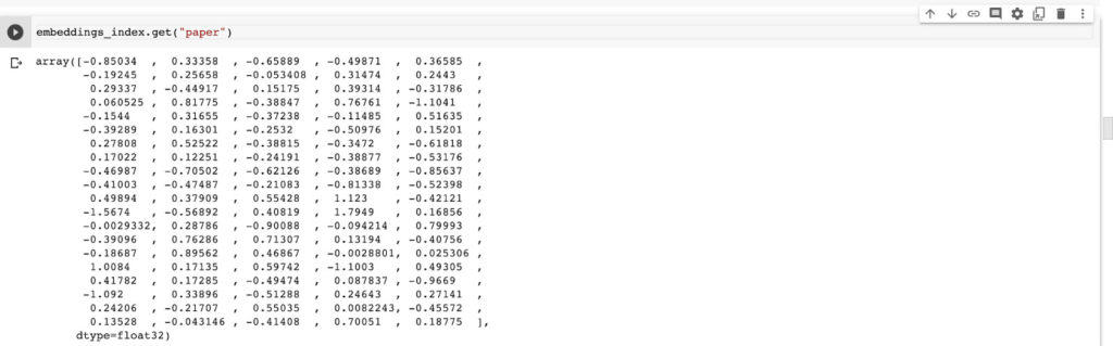
The next step is to create an embedding matrix for each word in the training set. The embedding vector for each word can be selected from the `embeddings_index` obtained above. For example, here is how the embedding for the word paper looks like.
embeddings_index.get("paper")
Let’s now obtain the embedding for every word in the training set. If an embedding for a certain word doesn’t exist, the embedding will be represented with zeros.
					embedding_matrix = np.zeros((len(word_index) + 1, max_length))
for word, i in word_index.items():
    embedding_vector = embeddings_index.get(word)
    if embedding_vector is not None:
        # words not found in embedding index will be all-zeros.
        embedding_matrix[i] = embedding_vector
Keras Embedding Layer
In the last section, you trained a custom embedding layer. Now that the embedding matrix has been obtained above, that process isn’t necessary. What’s needed here is the creation of an embedding layer with the embedding matrix obtained above. An embedding layer is therefore created and the embedding matrix obtained above is used as its weight. The `trainable` attribute of the layer is set to false so that the layer isn’t trained again. Otherwise, the layer will be trained again and all the pre-trained weights will be lost. The first argument is the size of the vocabulary, the `input_length` is the length of the input sequences while the `output_dim` is the dimension of the dense embedding.
					embedding_layer = Embedding(input_dim=len(word_index) + 1,
                            output_dim=max_length,
                            weights=[embedding_matrix],
                            input_length=max_length,
                            trainable=False)
Convolutional Neural Network for sentence classification
The next step is to create the convolutional neural network. The first layer is the embedding layer defined above. The other layers are similar to what you have already seen.
					model = Sequential([
    embedding_layer,
  Conv1D(128, 5, activation='relu'),
    GlobalMaxPooling1D(),
  Dense(10, activation='relu'),
  Dense(1, activation='sigmoid')
])
Convolutional Neural Networks for NLP
With this network in place, the next step is to prepare it for training. Since the problem is the same, the network is compiled with parameters similar to what we’ve used previously.
model.compile(loss='binary_crossentropy',optimizer='adam',metrics=['accuracy'])
Training CNN model
Let’s now fit this model to the training set. The model is trained for 20 epochs. You can implement the `EarlyStoppingCallback` to stop the training process once the model stops improving.
history = model.fit(X_train_padded, y_train, epochs=20, validation_data=(X_test_padded, y_test))
Evaluation
Let’s now check the performance of this model on the testing set. You can see that an improvement of 5% is achieved after employing the pre-trained GloVe embeddings.
					loss, accuracy = model.evaluate(X_test_padded,y_test)
print('Testing Accuracy is {} '.format(accuracy*100))

Hyperparameters Optimization
Throughout this article, you have defined all parameters manually. This process is not sustainable especially when you want to search for the parameters that result in a model with the highest accuracy. The solution is Hyperparameters Optimization. This is the process of searching for the best model parameters programmatically. Two common ways for doing this is random search and grid search. Random search uses the given parameters in a random manner while grid search performs an exhaustive search over the given parameters. Grid search is more resource-intensive because it is exhaustive. Let’s look at how grid search can be implemented.
Defining the model to be optimized
The easiest way to perform optimization in TensorFlow is to use a Scikit-learn wrapper that enables us to apply grid search to a neural network. That wrapper expects a model function definition. Let’s start by creating that function.
The model definition is similar to what you have used previously. Notice that the model is defined and then returned by the function.
					def model_to_optimize(num_filters, kernel_size):
  model = Sequential([
    embedding_layer,
    Conv1D(num_filters, kernel_size, activation='relu'),
    GlobalMaxPooling1D(),
    Dense(10, activation='relu'),
    Dense(1, activation='sigmoid')])
  model.compile(loss='binary_crossentropy',optimizer='adam',metrics=['accuracy'])
  return model
Creating the parameters grid
The next step is to define the parameters that you would like to perform an exhaustive search over. The parameters are defined in a Python dictionary.
					params = {
    "num_filters":[32, 64, 128],
    "kernel_size":[3, 5, 7],
}
Define the Keras Classifier
The next step is to define the model using the `KerasClassifier` wrapper function. The function expects:
- The model function defined above
- The number of epochs
- The batch size
					from tensorflow.keras.wrappers.scikit_learn import KerasClassifier
model = KerasClassifier(build_fn=model_to_optimize,
                            epochs=20,
                           batch_size=10,
                            verbose=False)
Performing grid search
Let’s now perform the grid search. The `GridSearchCV` expects:
- The model defined above
- The parameters defined above
- The `cv` that dictates how cross-validation will be performed. If none is defined, 5-fold cross-validation is used. If an integer is used, it defines the number of folds in a (Stratified)KFold.
The next step after creating an instance of `GridSearchCV` is to fit it to the training data.
					from sklearn.model_selection import GridSearchCV
search = GridSearchCV(estimator=model, param_grid=params,
                              cv=5, verbose=1)
search_result = search.fit(X_train_padded, y_train)
After the fitting is done, the accuracy can be obtained using the `score` method.
test_accuracy = search.score(X_test_padded, y_test)
You can also check for the parameter combination that resulted in the best results.
search.best_params_
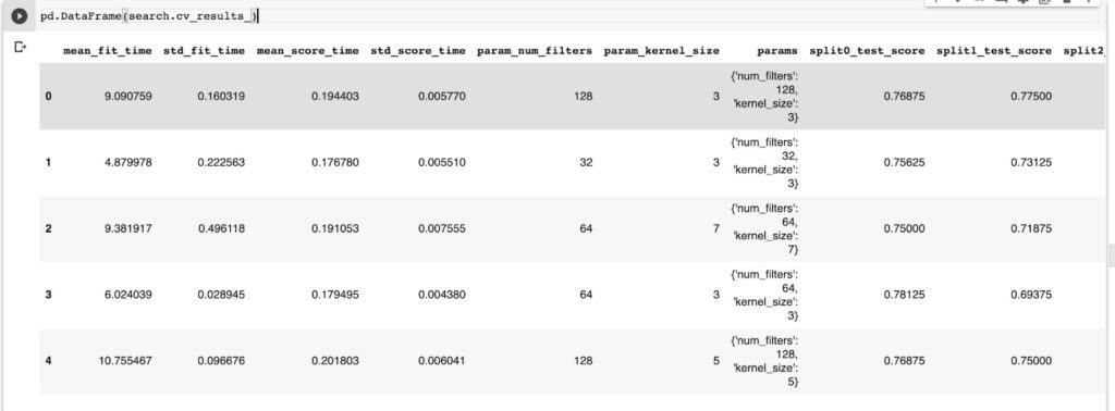
The other thing you can do is to check the cross-validated results.
pd.DataFrame(search.cv_results_)
That’s it folks for this section!
CNN for sentence classification with PyTorch
You can also perform text classification in PyTorch. Let’s look at that in action by building a simple Sequential model in PyTorch.
					import torch
from torch import nn
model = nn.Sequential(
          nn.Linear(X_train_s.shape[1], 64),
             nn.ReLU(),
             nn.Linear(64, 2),
             nn.Sigmoid()
        )
To keep things simple, let’s use the dataset that was processed using Scikit-learn. The data has to be converted to Torch tensors.
					X_train = torch.Tensor(X_train_s)
y_train = torch.LongTensor(y_train_s)
X_test = torch.Tensor(X_test_s)
y_test = torch.LongTensor(y_test_s)
The next step is to define the optimizer and the loss function that will be used by the PyTorch model.
					criterion = nn.CrossEntropyLoss()
optimizer = torch.optim.Adam(model.parameters(), lr=0.01)
Let’s now run this network for 50 epochs while displaying the loss for the even-numbered epochs.
					epochs = 50
losses = []

for i in range(epochs):
    i+=1
    y_pred = model.forward(X_train)
    loss = criterion(y_pred, y_train)
    losses.append(loss)

    if i%2 == 0:
        print(f'epoch: {i:2}  loss: {loss.item():10.8f}')

    optimizer.zero_grad()
    loss.backward()
    optimizer.step()
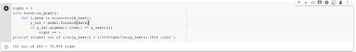
The next step is to use this model to make predictions on the test set.
					right = 0
with torch.no_grad():
    for i,data in enumerate(X_test):
        y_val = model.forward(data)
        if y_val.argmax().item() == y_test[i]:
            right += 1
print(f'{right} out of {len(y_test)} = {100*right/len(y_test):.2f}% right')
This simple model garners an accuracy of 75%.
A better way to perform text classification in PyTorch is to use its `torchtext` library. A thorough example of how to use the `torchtext` library for text classification has been provided by the official docs.
Deep learning architectures for text classification
Apart from Convolutional Neural neural networks, other network architectures can be used for text classification. They include:
- Recurrent Neural Networks (RNNs)
- Long Short Term Memory Networks (LSTMS)
- The Transformer Network
RNNs can handle sequence data because they can remember temporal information. An application of RNNs is the use of character-level RNNs to predict the next word in a sentence. RNNs can also be used in captioning images. Obviously, they can be used in sentence classification tasks such as sentiment classification. RNNs face two major issues, i.e the vanishing and exploding gradients problem. These issues are addressed by the LSTM network.
LSTMs are great at keeping long-term memory dependencies. They do this via a cell state. The cell state is updated with important information at every time step. The current input, the previous output, and the updated cell state are used for computing the output at each time step. The LSTM architecture does this using gates. Particularly it has the input gate, the forget gate, and the output gate.
The Transformer Network was introduced in this paper. It uses an encoder-decoder architecture that is similar to RNNs. The major difference from RNNs is the introduction of attention blocks. These blocks are responsible for computing the relationship between different words in the input. More attention is given to words that are highly related. Multiple attention blocks are used and the average of the computed correlation is taken. The network is great at maintaining context between different words. Some of the models implementing this architecture include BERT by Google and GPT by OpenAI.
One of the easiest ways to get started with these state-of-the-art NLP models is through the use of the `transformers` library from HuggingFace. For instance, you can use the library and use a pre-trained BERT model. Multiple other pre-trained models are also provided. The library provides support for PyTorch and TensorFlow.
10 applications of Artificial Neural Networks in natural language processing
In the last section, you have seen that multiple network architectures can be used for NLP tasks. The question that begs now is which are those NLP tasks. Let’s mention a couple here:
- Question answering. This involves extracting an answer from a text given a certain question.
- Text generation. Given a certain context, a neural network can generate a coherent and continuous piece of text.
- Text summarization. Neural networks can summary huge pieces of text.
- Named Entity Recognition. Given some sentences, a network can identify entities such as people, organizations, and locations.
- Translation. Neural networks are being used to translate text from one language to another.
- Text classification. This is the task of categorizing pieces of text into certain classes. For instance, sentiment analysis and spam detection.
- Part-of-Speech Tagging. This involves categorizing the part of speech a certain word or phrase belongs to. For instance, it could be a verb, an adjective, a pronoun, and so on.
- Paraphrase detection. This entails determining if two sentences have the same meaning.
- Speech recognition. Identifying the person who is speaking. This can be applied in virtual assistants, hands-free computing, and video games.
- Character recognition. Character recognition can be used in extracting information from written text and documents such as invoices.
Best practices for text classification with deep learning
Now that you know which NLP tasks to apply neural networks to, let’s look at some of the best practices to keep in mind:
- Use pre-trained word embeddings. These will save you the time you would spend training custom word embeddings. Pre-trained word embeddings have also been proven to perform better.
- Perform parameter optimization. Using a technique such as grid search or random search can enable you to quickly arrive at the optimal parameters for your NLP model.
- Quality training data. Neural networks, in general, perform better with lots of data. If you are not getting great results, consider collecting more data.
- Go deeper. For text classification models, try a deeper model if not getting good results on a shallow network.
Final thoughts
In this article, we have covered the nuts and bolts of tackling a text classification problem using deep learning. You have seen that the handling of text data is very different from that of normal numerical data. Essentially, you had to convert the text data into a numerical form that could be understood by the machine learning and deep learning model. In the course of the article, you have also gone through several examples of applying deep learning to text classification problems. Specifically, you have covered:
- How to create a baseline model for text classification
- Processing text data for NLP models
- How Convolutional Neural Networks work in the context of NLP tasks
- Building NLP models in TensorFlow and PyTorch
- Training a word embedding for text classification
- How to apply Convolutional Neural Networks to text classification problems
- Using pre-trained GloVe word embeddings for text classification
- Best practices for text classification in deep learning
..and so much more.
For an end to end example of an NLP problem, you can watch our webinar on how to build an NLP pipeline with BERT in PyTorch.
Resources
Deep Learning for NLP Best Practices
A Complete Guide to CNN for Sentence Classification with PyTorch
Understanding Convolutional Neural Networks for NLP
Convolutional Neural Networks for Text Classification
Convolutional Neural Networks for Sentence Classification Paper
Text Classification: All Tips and Tricks from 5 Kaggle Competitions